education <- read.csv("data/education_intervention.csv")

table(education$school_id)
S01 S02 S03 S04 S05 S06 S07 S08 S09 S10 S11 S12
20 21 25 19 18 21 25 25 23 22 20 22 Partial pooling for nested social science and education data
By the end of this module, participants should be able to:
Education and social-science data are routinely nested. Learners sit inside classrooms inside schools inside districts. Patients sit inside clinics inside hospitals. Survey respondents sit inside neighbourhoods inside regions. The nesting matters: outcomes for units inside the same group are more similar to each other than to units in other groups, and a model that ignores this gets the uncertainty wrong even when the point estimates look reasonable.
In the education dataset, learners are nested within schools. Endline scores may vary by school for reasons that the researcher cannot fully observe: leadership, resources, peer composition, neighbourhood context, the chemistry of a particular teacher with a particular cohort. These unmeasured factors push learners at the same school toward similar outcomes, regardless of any individual-level predictors the model controls for.
education <- read.csv("data/education_intervention.csv")
table(education$school_id)
S01 S02 S03 S04 S05 S06 S07 S08 S09 S10 S11 S12
20 21 25 19 18 21 25 25 23 22 20 22 The school-level count is the first diagnostic. If most schools have 20 or more learners, the school-specific estimates will be reasonably stable. If many schools have only 3 or 4 learners, the estimates for those schools will be highly uncertain when fitted separately, which is exactly the situation hierarchical modelling is designed for.
There are three modelling strategies for nested data, and the contrast between them is the conceptual core of hierarchical models. The first two are limiting cases; the third is the one that almost always answers the applied question.
Ignore school differences entirely:
endline_score ~ intervention + baseline_score + ses_indexThis treats every learner as exchangeable, as if school membership carried no information. The model gets the population-level coefficients but understates uncertainty, because residuals from learners at the same school are not independent. Reviewers will object, and they will be right.
Estimate each school separately by including school as a fixed effect:
endline_score ~ school_idThis honours the school structure but in the most expensive way. Each school gets its own intercept estimated from its own learners alone. Schools with 4 learners get noisy estimates, and the model has no mechanism to recognise that those noisy estimates are likely too extreme. The model also makes no claim about the population of schools: there are simply 30 schools, each with its own number.
Estimate school-level variation by modelling schools as draws from a common distribution:
endline_score ~ intervention + baseline_score + ses_index + (1 | school_id)This is the hierarchical model. The (1 | school_id) term says that each school has its own intercept, but those intercepts are themselves drawn from a normal distribution whose mean and standard deviation are estimated from the data. The consequence is that school-specific estimates are shrunk toward the overall mean by an amount that depends on how much information each school provides. A school with 4 learners gets pulled strongly toward the average; a school with 40 learners moves much less. This is partial pooling, and it is the strategy that gives hierarchical models their statistical efficiency.
The brms formula syntax for the hierarchical model is one term longer than the standard regression: the (1 | school_id) adds school-specific intercepts. The priors now include one additional class, prior(exponential(1), class = "sd"), which is the prior on the school-level standard deviation. This is a new modelling decision and deserves its own consideration. An Exponential(1) prior on the school-level SD pulls weakly toward smaller values; a flat prior would allow implausibly large between-school variation and a tighter prior would force the school estimates to look more similar than the data warrant. The choice should be defended against the substantive expectation about how much schools differ on this outcome.
library(brms)

hier_model <- brm(
  endline_score ~ intervention + baseline_score + ses_index + (1 | school_id),
  data = education,
  family = gaussian(),
  prior = c(
    prior(normal(60, 15), class = "Intercept"),
    prior(normal(0, 10), class = "b", coef = "intervention"),
    prior(normal(0.6, 0.2), class = "b", coef = "baseline_score"),
    prior(normal(0, 4), class = "b", coef = "ses_index"),
    prior(exponential(1), class = "sd"),
    prior(exponential(1), class = "sigma")
  ),
  backend = "cmdstanr",
  chains = 4,
  cores = 4,
  iter = 2000,
  seed = 2026
)A hierarchical model returns two interesting things at once: the population-level coefficients (intervention, baseline, SES), and the school-specific deviations from the overall intercept. The school deviations tell the researcher which schools are doing better or worse than the average after accounting for learner-level predictors, and they come with credible intervals that reflect both the sample size at each school and the partial-pooling shrinkage. A school with few learners will have a wider credible interval and an estimate closer to zero.
school_effects <- ranef(hier_model)$school_id[, , "Intercept"]

school_effects

dotchart(
  school_effects[, "Estimate"],
  labels = rownames(school_effects),
  xlab = "School effect"
)

abline(v = 0, lty = 2)school_means <- aggregate(
endline_score ~ school_id,
data = education,
FUN = mean
)
school_means$n <- as.integer(table(education$school_id)[school_means$school_id])
overall_mean <- mean(education$endline_score)
plot(
school_means$endline_score,
seq_along(school_means$school_id),
cex = sqrt(school_means$n) / 3,
pch = 19,
xlab = "Raw school mean endline score",
ylab = "School"
)
abline(v = overall_mean, lty = 2)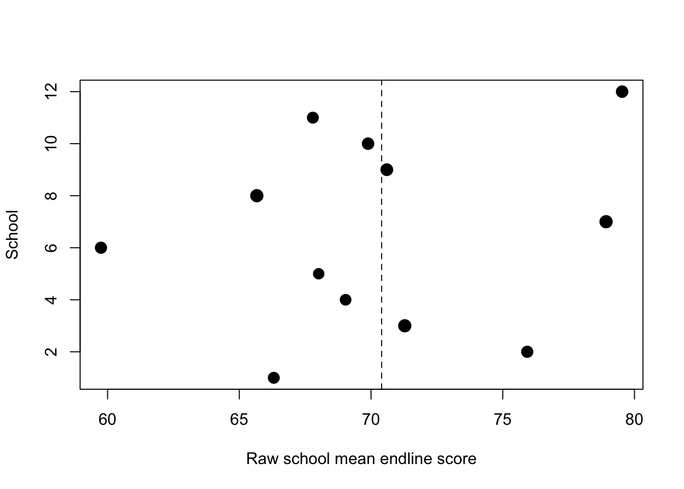
The point size encodes the number of learners at each school. The dashed vertical line is the overall sample mean. Schools far from this line are the candidates for “doing better” or “doing worse” than the average, but the visual is misleading if read directly: schools represented by the smallest dots are also the ones whose raw means are least reliable. Raw school means are not the same as hierarchical posterior estimates. The hierarchical model takes exactly this information and produces a more honest version: each school’s estimate is pulled toward the overall mean by an amount proportional to how little data that school provides. A school with 4 learners whose raw mean is 85 will end up with a posterior estimate noticeably closer to the overall average, with a credible interval that reflects the small sample.
This shrinkage is sometimes mistaken for an inappropriate flattening of real differences. It is the opposite. The hierarchical model is saying: a raw mean of 85 from 4 learners is weak evidence that the school is genuinely outperforming the average, and the model produces an estimate that takes that weakness into account. If the school really is exceptional, more data will move the posterior. If it is not, the posterior remains close to the average and the analyst avoids being fooled by noise.
We fitted a Bayesian varying-intercept model with learners nested within schools. The model estimated the intervention effect while allowing baseline achievement to vary across schools through school-level intercepts. The posterior distribution of the school-level standard deviation indicated [small/moderate/large] between-school variation after accounting for learner-level predictors.
Hierarchical models are one of the strongest reasons applied researchers should learn Bayesian analysis. They estimate group-level variation while avoiding the instability of separate estimates for every group, and they propagate the resulting uncertainty into the population-level coefficients in a way that single-level models cannot. In Bayesian form they also accept priors on the group-level standard deviation, which gives the analyst explicit control over how much between-group variation the model treats as plausible. The same workflow extends to crossed and three-level structures, but the two-level case covered here is the building block.