Translating familiar regression into posterior inference
1 Learning Outcomes
By the end of this module, participants should be able to:
Read a regression result as an answer to an education research question.
Interpret posterior means, credible intervals, and decision-relevant probabilities.
Compare familiar regression language with Bayesian reporting language.
Report whether an intervention effect is likely to be educationally meaningful.
2 Research Scenario
The research question for this notebook is whether an education intervention improves endline achievement once baseline score and socioeconomic status have been accounted for. The question is familiar to applied researchers because it is exactly the question a linear regression with three predictors normally addresses. What changes is the inferential machinery surrounding it, not the model structure itself.
The same dataset was used in notebook 02 to anchor prior choices. The descriptive summary below is included here as a reminder of the scale on which every coefficient will be interpreted.
 endline_score     intervention    baseline_score    ses_index
 Min.   : 34.72   Min.   :0.0000   Min.   :25.65   Min.   :-2.20000
 1st Qu.: 61.71   1st Qu.:0.0000   1st Qu.:51.51   1st Qu.:-0.58800
 Median : 70.47   Median :1.0000   Median :58.63   Median : 0.01700
 Mean   : 70.40   Mean   :0.5057   Mean   :58.03   Mean   :-0.01687
 3rd Qu.: 78.38   3rd Qu.:1.0000   3rd Qu.:65.84   3rd Qu.: 0.55800
 Max.   :100.00   Max.   :1.0000   Max.   :93.74   Max.   : 2.20000
 attendance_rate
 Min.   : 62.19
 1st Qu.: 79.34
 Median : 84.39
 Mean   : 84.32
 3rd Qu.: 89.42
 Max.   :100.00
3 Frequentist Baseline
A frequentist linear regression is the natural baseline. Fitting it first is useful for two reasons. It produces familiar numbers that anchor expectations for what the Bayesian model will return, and it makes the inferential difference between the two approaches visible by direct comparison rather than by argument.
Read the coefficient table substantively. The intervention coefficient is the estimated mean difference in endline score between treated and comparison learners after adjusting for baseline and SES. A positive estimate around 4 to 5 points, with a confidence interval that does not include zero, is the kind of result a frequentist analysis would describe as “statistically significant.” The baseline coefficient near 0.85 says that a one-point higher baseline score is associated with roughly 0.85 points higher endline, which is the autoregression that dominates this kind of education data. The SES coefficient is smaller and noisier.
For this audience, the important limitation is not that the frequentist regression is wrong. It is that the table does not directly answer two decision-facing questions: how probable is it that the intervention effect is positive, and how probable is it that the effect is larger than a practical threshold such as 3 score points? The Bayesian model fitted next returns those quantities directly.
4 Bayesian Model
The Bayesian model uses exactly the same likelihood structure as the frequentist one:
Here, \(Y_i\) is learner \(i\)’s endline score, \(I_i\) indicates whether the learner received the intervention, \(B_i\) is the baseline score, and \(S_i\) is the standardised SES index.
The change is that every parameter now needs a prior. Each prior is chosen with reference to the scale of the outcome and the substantive expectations discussed in notebook 02:
Each line is a statement about the parameter on the score-point scale. The intercept prior Normal(60, 15) says that, for a hypothetical learner with intervention = 0, baseline = 0, and SES = 0, the expected endline score is around 60, with a plausible range from roughly 30 to 90. That range covers the observed score distribution and rules out impossible values like 200. The Normal(0, 10) on the intervention coefficient is the weakly informative prior from notebook 02: zero is the prior best guess, but effects up to about 20 points either way are not ruled out. The baseline coefficient prior Normal(0.6, 0.2) reflects strong prior evidence that baseline scores predict endline scores with a slope between roughly 0.2 and 1.0. The SES prior Normal(0, 4) allows a moderate effect in either direction. The residual standard deviation sigma is given an Exponential(1) prior, which keeps it positive and weakly pulls it toward smaller values.
These priors are defensible because they sit on the scale of the actual outcome and because each one corresponds to a substantive claim that could be challenged on substantive grounds. A reviewer who disagrees with the baseline-prior centre of 0.6 has a specific number to argue with, not a vague philosophical objection.
5 Bayesian Regression Results
The model is fitted in brms. This is the main code participants need to copy if they want to run the Bayesian regression.
library(brms)priors <-c(prior(normal(60, 15), class ="Intercept"),prior(normal(0, 10), class ="b", coef ="intervention"),prior(normal(0.6, 0.2), class ="b", coef ="baseline_score"),prior(normal(0, 4), class ="b", coef ="ses_index"),prior(exponential(1), class ="sigma"))bayes_model <-brm( endline_score ~ intervention + baseline_score + ses_index,data = education,family =gaussian(),prior = priors,backend ="cmdstanr",chains =4,cores =4,iter =2000,seed =2026,refresh =0)
summary(bayes_model)
 Family: gaussian
  Links: mu = identity
Formula: endline_score ~ intervention + baseline_score + ses_index
   Data: education (Number of observations: 261)
  Draws: 4 chains, each with iter = 2000; warmup = 1000; thin = 1;
         total post-warmup draws = 4000

Regression Coefficients:
               Estimate Est.Error l-95% CI u-95% CI Rhat Bulk_ESS Tail_ESS
Intercept         19.10      2.65    13.87    24.25 1.00     4007     3345
intervention       4.86      0.81     3.24     6.36 1.00     4999     2977
baseline_score     0.84      0.04     0.76     0.93 1.00     4047     3263
ses_index          1.93      0.55     0.84     3.00 1.00     4116     3502

Further Distributional Parameters:
      Estimate Est.Error l-95% CI u-95% CI Rhat Bulk_ESS Tail_ESS
sigma     6.72      0.30     6.16     7.36 1.00     4756     3182

Draws were sampled using sample(hmc). For each parameter, Bulk_ESS
and Tail_ESS are effective sample size measures, and Rhat is the potential
scale reduction factor on split chains (at convergence, Rhat = 1).
Read this as a regression table in score points. The intervention row is the central row for the education question. The posterior mean is the estimated score difference after accounting for baseline score and SES. The credible interval gives the range of plausible intervention effects under the model and priors. Rhat is included as a basic computation check; values close to 1 indicate that the chains agree.
6 Posterior Interpretation
The regression table gives the estimated effect and its plausible range. The Bayesian payoff is that we can also ask decision-facing probability questions directly.
posterior_draws <- posterior::as_draws_df(bayes_model)intervention_effect <- posterior_draws$b_interventionposterior_summary(bayes_model, pars ="b_intervention")
Each column corresponds to a different kind of substantive claim. The posterior mean is the central estimate. The 95% credible range describes plausible values under the model. The last two columns answer the practical questions directly: how likely is it that the intervention helps at all, and how likely is it that the effect exceeds the 3-point threshold used here as a minimum meaningful gain?
The framing here matters. In a frequentist analysis, the question “what is the probability that the intervention helps?” is not a question the framework answers directly. In the Bayesian analysis, the probability is a direct property of the posterior. Here, the result supports a direct applied claim: under this model and these priors, the intervention is very likely to improve endline scores by an educationally meaningful amount.
7 Posterior Plot
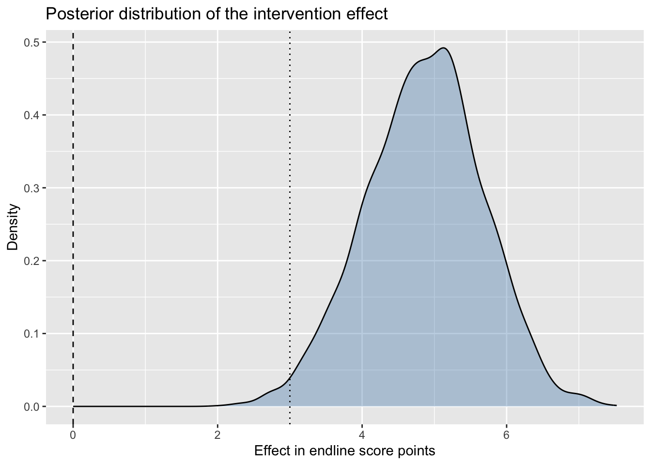
A density plot of the posterior makes the probability statements above visible at a glance. The dashed line at zero divides effects that hurt from effects that help; the area of the curve to the right of zero is prob_positive. The dotted line at 3 marks the practical threshold; the area to the right of that line is prob_practical. A reader can see the answer without computing it.
ggplot(posterior_draws, aes(x = b_intervention)) +geom_density(fill ="steelblue", alpha =0.35) +geom_vline(xintercept =0, linetype ="dashed") +geom_vline(xintercept =3, linetype ="dotted") +labs(title ="Posterior distribution of the intervention effect",x ="Effect in endline score points",y ="Density" )
Posterior density plots are the workhorse figure for Bayesian results. They show the central estimate, the uncertainty, and the position of any substantively important threshold in one image. They are also easy to misread, in two ways. A wide posterior is not the same as no effect; it is genuine uncertainty about a quantity that may still be entirely on one side of zero. And a narrow posterior is not certainty about reality; it is certainty conditional on this model and these priors. Reporting the figure alongside the prior choices and the convergence diagnostics is what licenses the inference.
8 Posterior Predictions
Coefficient summaries are useful, but applied audiences usually understand predicted outcomes more readily. The same posterior can be used to compare two otherwise similar learners: both have average baseline achievement and average SES, but only one receives the intervention.
The difference between the two rows is the intervention effect expressed in the original score units. This is often the most useful way to communicate the result to a district official or programme team: not as a coefficient table first, but as the expected difference in scores for comparable learners.
9 Exercise
Using the Bayesian model:
Estimate the posterior probability that the intervention effect is positive.
Estimate the posterior probability that the intervention effect is greater than 3 points.
Create a posterior density plot.
Write a results paragraph for an applied education report.
10 Reporting Template
The posterior mean intervention effect was [X] score points, with a 95% credible interval from [L] to [U]. The posterior probability that the intervention improved scores was [P1], and the probability that the effect exceeded the practical threshold of 3 points was [P2]. These results suggest [interpretation in substantive language].
For a social-science or public-facing report, the same result can be written with less statistical language:
Learners who received the intervention were expected to score about [X] points higher than comparable learners who did not receive it, after accounting for baseline achievement and socioeconomic status. The plausible range of improvement was from [L] to [U] points. The evidence strongly suggests that the intervention improved scores, and there was [P2] probability that the improvement was at least 3 points, the threshold used here for a practically meaningful gain. These results suggest [interpretation in substantive language].
11 Takeaway
Bayesian regression uses familiar model structures and changes the inferential output. The same lm-style formula and the same linear predictor produce posterior distributions instead of point estimates. Those posteriors can be summarised flexibly: by their means, by their credible intervals, by the probability they place on substantively important thresholds, or by the predicted outcomes they imply for hypothetical cases. The next notebook extends this exact workflow to binary and ordinal outcomes; the workflow does not change, only the likelihood does.
Source Code
---title: "03 Bayesian Linear Regression"subtitle: "Translating familiar regression into posterior inference"format: html: toc: true number-sections: trueexecute: warning: false message: false---```{=html}<nav class="module-route" aria-label="Notebook route"> <a href="01_bayesian_reasoning.html">01<br>Reasoning</a> <a href="02_priors.html">02<br>Priors</a> <a class="active" href="03_bayesian_regression.html">03<br>Regression</a> <a href="04_binary_and_ordinal_models.html">04<br>GLMs</a> <a href="05_hierarchical_models.html">05<br>Multilevel</a> <a href="06_model_checking.html">06<br>Checking</a> <a href="07_reporting.html">07<br>Reporting</a></nav>```## Learning OutcomesBy the end of this module, participants should be able to:1. Read a regression result as an answer to an education research question.2. Interpret posterior means, credible intervals, and decision-relevant probabilities.3. Compare familiar regression language with Bayesian reporting language.4. Report whether an intervention effect is likely to be educationally meaningful.## Research ScenarioThe research question for this notebook is whether an education intervention improves endline achievement once baseline score and socioeconomic status have been accounted for. The question is familiar to applied researchers because it is exactly the question a linear regression with three predictors normally addresses. What changes is the inferential machinery surrounding it, not the model structure itself.The same dataset was used in notebook 02 to anchor prior choices. The descriptive summary below is included here as a reminder of the scale on which every coefficient will be interpreted.```{r}library(readr)library(ggplot2)education <-read_csv("data/education_intervention.csv")summary(education[c("endline_score","intervention","baseline_score","ses_index","attendance_rate")])```## Frequentist BaselineA frequentist linear regression is the natural baseline. Fitting it first is useful for two reasons. It produces familiar numbers that anchor expectations for what the Bayesian model will return, and it makes the inferential difference between the two approaches visible by direct comparison rather than by argument.```{r}freq_model <-lm( endline_score ~ intervention + baseline_score + ses_index,data = education)summary(freq_model)``````{r}anova(freq_model)confint(freq_model)```Read the coefficient table substantively. The intervention coefficient is the estimated mean difference in endline score between treated and comparison learners after adjusting for baseline and SES. A positive estimate around 4 to 5 points, with a confidence interval that does not include zero, is the kind of result a frequentist analysis would describe as "statistically significant." The baseline coefficient near 0.85 says that a one-point higher baseline score is associated with roughly 0.85 points higher endline, which is the autoregression that dominates this kind of education data. The SES coefficient is smaller and noisier.For this audience, the important limitation is not that the frequentist regression is wrong. It is that the table does not directly answer two decision-facing questions: how probable is it that the intervention effect is positive, and how probable is it that the effect is larger than a practical threshold such as 3 score points? The Bayesian model fitted next returns those quantities directly.## Bayesian ModelThe Bayesian model uses exactly the same likelihood structure as the frequentist one:$$\begin{aligned}Y_i &\sim \mathrm{Normal}(\mu_i, \sigma), \\\mu_i &= \alpha + \beta_{\mathrm{intervention}} I_i + \beta_{\mathrm{baseline}} B_i + \beta_{\mathrm{SES}} S_i .\end{aligned}$$Here, $Y_i$ is learner $i$'s endline score, $I_i$ indicates whether the learner received the intervention, $B_i$ is the baseline score, and $S_i$ is the standardised SES index.The change is that every parameter now needs a prior. Each prior is chosen with reference to the scale of the outcome and the substantive expectations discussed in notebook 02:$$\begin{aligned}\alpha &\sim \mathrm{Normal}(60, 15), \\\beta_{\mathrm{intervention}} &\sim \mathrm{Normal}(0, 10), \\\beta_{\mathrm{baseline}} &\sim \mathrm{Normal}(0.6, 0.2), \\\beta_{\mathrm{SES}} &\sim \mathrm{Normal}(0, 4), \\\sigma &\sim \mathrm{Exponential}(1).\end{aligned}$$Each line is a statement about the parameter on the score-point scale. The intercept prior `Normal(60, 15)` says that, for a hypothetical learner with intervention = 0, baseline = 0, and SES = 0, the expected endline score is around 60, with a plausible range from roughly 30 to 90. That range covers the observed score distribution and rules out impossible values like 200. The `Normal(0, 10)` on the intervention coefficient is the weakly informative prior from notebook 02: zero is the prior best guess, but effects up to about 20 points either way are not ruled out. The baseline coefficient prior `Normal(0.6, 0.2)` reflects strong prior evidence that baseline scores predict endline scores with a slope between roughly 0.2 and 1.0. The SES prior `Normal(0, 4)` allows a moderate effect in either direction. The residual standard deviation `sigma` is given an `Exponential(1)` prior, which keeps it positive and weakly pulls it toward smaller values.These priors are defensible because they sit on the scale of the actual outcome and because each one corresponds to a substantive claim that could be challenged on substantive grounds. A reviewer who disagrees with the baseline-prior centre of 0.6 has a specific number to argue with, not a vague philosophical objection.## Bayesian Regression ResultsThe model is fitted in `brms`. This is the main code participants need to copy if they want to run the Bayesian regression.```{r}#| results: hide#| message: false#| warning: falselibrary(brms)priors <-c(prior(normal(60, 15), class ="Intercept"),prior(normal(0, 10), class ="b", coef ="intervention"),prior(normal(0.6, 0.2), class ="b", coef ="baseline_score"),prior(normal(0, 4), class ="b", coef ="ses_index"),prior(exponential(1), class ="sigma"))bayes_model <-brm( endline_score ~ intervention + baseline_score + ses_index,data = education,family =gaussian(),prior = priors,backend ="cmdstanr",chains =4,cores =4,iter =2000,seed =2026,refresh =0)``````{r}summary(bayes_model)```Read this as a regression table in score points. The intervention row is the central row for the education question. The posterior mean is the estimated score difference after accounting for baseline score and SES. The credible interval gives the range of plausible intervention effects under the model and priors. `Rhat` is included as a basic computation check; values close to 1 indicate that the chains agree.## Posterior InterpretationThe regression table gives the estimated effect and its plausible range. The Bayesian payoff is that we can also ask decision-facing probability questions directly.```{r}posterior_draws <- posterior::as_draws_df(bayes_model)intervention_effect <- posterior_draws$b_interventionposterior_summary(bayes_model, pars ="b_intervention")c(probability_positive =mean(intervention_effect >0),probability_above_3_points =mean(intervention_effect >3))```Each column corresponds to a different kind of substantive claim. The posterior mean is the central estimate. The 95% credible range describes plausible values under the model. The last two columns answer the practical questions directly: how likely is it that the intervention helps at all, and how likely is it that the effect exceeds the 3-point threshold used here as a minimum meaningful gain?The framing here matters. In a frequentist analysis, the question "what is the probability that the intervention helps?" is not a question the framework answers directly. In the Bayesian analysis, the probability is a direct property of the posterior. Here, the result supports a direct applied claim: under this model and these priors, the intervention is very likely to improve endline scores by an educationally meaningful amount.## Posterior PlotA density plot of the posterior makes the probability statements above visible at a glance. The dashed line at zero divides effects that hurt from effects that help; the area of the curve to the right of zero is `prob_positive`. The dotted line at 3 marks the practical threshold; the area to the right of that line is `prob_practical`. A reader can see the answer without computing it.```{r}ggplot(posterior_draws, aes(x = b_intervention)) +geom_density(fill ="steelblue", alpha =0.35) +geom_vline(xintercept =0, linetype ="dashed") +geom_vline(xintercept =3, linetype ="dotted") +labs(title ="Posterior distribution of the intervention effect",x ="Effect in endline score points",y ="Density" )```Posterior density plots are the workhorse figure for Bayesian results. They show the central estimate, the uncertainty, and the position of any substantively important threshold in one image. They are also easy to misread, in two ways. A wide posterior is not the same as no effect; it is genuine uncertainty about a quantity that may still be entirely on one side of zero. And a narrow posterior is not certainty about reality; it is certainty conditional on this model and these priors. Reporting the figure alongside the prior choices and the convergence diagnostics is what licenses the inference.## Posterior PredictionsCoefficient summaries are useful, but applied audiences usually understand predicted outcomes more readily. The same posterior can be used to compare two otherwise similar learners: both have average baseline achievement and average SES, but only one receives the intervention.```{r}new_learners <-data.frame(intervention =c(0, 1),baseline_score =mean(education$baseline_score),ses_index =0)fitted(bayes_model, newdata = new_learners)```The difference between the two rows is the intervention effect expressed in the original score units. This is often the most useful way to communicate the result to a district official or programme team: not as a coefficient table first, but as the expected difference in scores for comparable learners.## ExerciseUsing the Bayesian model:1. Estimate the posterior probability that the intervention effect is positive.2. Estimate the posterior probability that the intervention effect is greater than 3 points.3. Create a posterior density plot.4. Write a results paragraph for an applied education report.## Reporting Template> The posterior mean intervention effect was [X] score points, with a 95% credible interval from [L] to [U]. The posterior probability that the intervention improved scores was [P1], and the probability that the effect exceeded the practical threshold of 3 points was [P2]. These results suggest [interpretation in substantive language].For a social-science or public-facing report, the same result can be written with less statistical language:> Learners who received the intervention were expected to score about [X] points higher than comparable learners who did not receive it, after accounting for baseline achievement and socioeconomic status. The plausible range of improvement was from [L] to [U] points. The evidence strongly suggests that the intervention improved scores, and there was [P2] probability that the improvement was at least 3 points, the threshold used here for a practically meaningful gain. These results suggest [interpretation in substantive language].## TakeawayBayesian regression uses familiar model structures and changes the inferential output. The same `lm`-style formula and the same linear predictor produce posterior distributions instead of point estimates. Those posteriors can be summarised flexibly: by their means, by their credible intervals, by the probability they place on substantively important thresholds, or by the predicted outcomes they imply for hypothetical cases. The next notebook extends this exact workflow to binary and ordinal outcomes; the workflow does not change, only the likelihood does.```{=html}<nav class="module-nav" aria-label="Module navigation"> <a href="02_priors.html">← Previous: Priors</a> <a href="04_binary_and_ordinal_models.html">Next: Binary and Ordinal →</a></nav>```