01 Bayesian Reasoning for Frequentist Researchers

From significance decisions to programme decisions under uncertainty

1 Learning Outcomes

By the end of this session, you should be able to:

Translate an education research decision into a probability question.
Identify the unknown quantity a study is trying to learn about.
Treat prior evidence as a transparent research judgement rather than a hidden assumption.
Use a simple pilot study to update uncertainty about whether a programme is likely to meet a meaningful benchmark.

2 The Programme Decision

A district has piloted a reading support programme with 30 learners. At the end of the pilot, 21 learners reached the agreed reading proficiency benchmark. The district now has to decide what to do next.

Discuss first

Is this programme promising enough to continue, adapt, or scale?

Details

That is not only a statistical question. It is a research judgement under uncertainty. The observed pilot result is encouraging, but 30 learners is a small group. The researcher has to decide what can be said responsibly about the larger population of similar learners who might receive the programme next year.

The headline figure is the observed pilot rate:

successes <- 21
n <- 30
successes / n

[1] 0.7

Discuss first

What does the observed 70% tell us, and what does it not tell us?

Details

Seventy per cent of the pilot learners reached the benchmark. That number is useful, but it is not the answer to the district’s question. The district is not asking only what happened among these 30 learners. It is asking what is likely to happen if the programme is used with future learners in the same kind of setting.

Bayesian decision question

What is the probability that the true benchmark success rate for this programme is above a minimum useful level, such as 60%?

Discuss first

What are the three parts of this question?

Details

The question can be unpacked in three parts.

The programme outcome is learners reaching the reading proficiency benchmark.

The unknown quantity is the success rate we would expect among similar learners beyond this pilot.

The decision line is 60%, the minimum rate being used here as a first marker of educational usefulness.

Bayesian analysis gives us a way to move from the pilot result to this kind of decision question.

Details

Bayesian analysis helps organise that judgement. The prior records what was plausible before the pilot. The likelihood represents what the pilot data support. The posterior summarises what is now plausible after both sources of evidence have been considered.

3 The Shift

Frequentist methods are useful, and they remain central to education research. They help researchers test clearly stated hypotheses, estimate uncertainty with confidence intervals, and avoid overclaiming from small studies. The shift in this workshop is not from “wrong” methods to “right” methods. It is from one kind of question to another.

In a hypothesis test, the p-value is attached to a specific null hypothesis, often a hypothesis about a parameter. In many education studies, the usual null says that an effect, difference, association, or parameter is zero.

For example, suppose an education researcher estimates a simple regression comparing learners who received a reading intervention with learners who did not:

\[ Y_i = \beta_0 + \beta_1 D_i + \varepsilon_i. \]

Here, $Y_i$ is learner $i$’s reading outcome and $D_i$ indicates whether learner $i$ received the intervention. The coefficient $\beta_1$ is the estimated difference associated with the intervention. The usual null hypothesis is:

\[ H_0 : \beta_1 = 0. \]

In words, the null says that the intervention coefficient is zero: no average difference in the reading outcome between the intervention and comparison groups, according to this model. A two-sided alternative would usually be written as:

\[ H_1 : \beta_1 \neq 0. \]

The p-value then measures how unusual the observed data, or a result at least as extreme, would be if that zero-effect null model were true.

The key shift

Frequentist framing:

“If the programme’s true success rate were 60%, how unusual would the eventual pilot result be once we observe how many learners reach the benchmark?”

Bayesian framing:

“After the pilot data are observed, what do we then believe about $\theta$, the programme’s true success rate among similar learners?”

Before the intervention is run, the result is not known. If the planned pilot includes 30 learners, we can write the future number of learners who reach the benchmark as $X$. Once the pilot has been completed, the observed count will be written as $x_{\text{obs}}$, and the observed success rate will be:

\[ \hat{\theta} = \frac{x_{\text{obs}}}{30}. \]

The district is not only interested in the eventual sample rate from those 30 learners. It wants to know what is plausible for the larger group of similar learners who might receive the programme in future.

For the benchmark-rate question, we can write the unknown programme success rate as $\theta$. If 60% is the minimum useful rate, a frequentist one-sided test could be written as:

\[ \begin{aligned} H_0 &: \theta = 0.60, \\ H_1 &: \theta > 0.60. \end{aligned} \]

For that test, the p-value is calculated after the pilot result is observed. If the observed count is $x_{\text{obs}}$, the p-value asks how unusual it would be to see $x_{\text{obs}}$ or more successes out of 30 learners if the true success rate were really 0.60:

\[ p = \Pr\left(X \geq x_{\text{obs}} \mid X \sim \mathrm{Binomial}(30, 0.60)\right). \]

A frequentist analysis can test whether the eventual pilot result is compatible with a threshold such as 60%, or it can provide a confidence interval for the success rate after the data are collected. These are useful tools. However, they do not directly say, “There is a given probability that the true success rate is above 60%.” A Bayesian analysis can express that uncertainty directly, conditional on the model and prior assumptions.

Careful wording for education researchers

Do not say: “The p-value is the probability that the intervention does not work.”
Rather say: “The p-value describes how unusual the observed data would be if the null model were true.”
Do not say: “Bayesian analysis proves the programme works.”
Rather say: “Bayesian analysis estimates how plausible different success rates are after considering the data and assumptions.”

Once the pilot has been run, Bayesian analysis does not treat the observed sample rate as the final truth. It treats the observed result as evidence that updates uncertainty about the programme’s true success rate. The posterior probability that the true success rate exceeds 60% provides a direct way of expressing how promising the programme appears, while still acknowledging uncertainty.

4 Prior Evidence, New Data, Updated Judgement

An education researcher rarely begins with no context. Before the pilot is run, there may already be evidence from earlier evaluations, teacher reports, implementation records, curriculum alignment, learner profiles, or experience with similar programmes. These things do not settle the question, but they shape what would count as a surprising or unsurprising result.

Bayesian analysis gives that ordinary research judgement a clear structure. It asks three practical questions.

Before the pilot

What seemed plausible?

The district may have little previous evidence, reasons for caution because implementation was uneven, or good evidence from a similar setting.

little previous evidence
implementation concerns
promising evidence from a similar context

Pilot evidence

What did the pilot add?

If 21 out of 30 learners reached the benchmark, the result is encouraging. But the observed 70% is not the final answer. It is evidence about what might happen with similar learners in future.

Updated judgement

How should the judgement change?

The updated judgement should speak directly to the education decision: how plausible is it that the programme would clear a meaningful benchmark, such as 60%, if used with similar learners?

Main point

Bayesian analysis is not asking education researchers to replace their research questions with statistical machinery. It asks them to make their starting assumptions visible, let the new data change those assumptions, and report the resulting uncertainty in a form that speaks directly to the programme decision.

5 A Practical Updating Model

For a benchmark outcome, each learner either reached the proficiency benchmark or did not. A simple model for this kind of outcome is:

successes ~ Binomial(n, theta)
theta ~ Beta(a, b)

The first line says that the number of learners meeting the benchmark is modelled as a count out of n learners, governed by the unknown programme rate theta. The second line says that our prior uncertainty about theta is represented with a beta distribution.

For this first example, the research interpretation matters more than the technical name. The two beta parameters, a and b, can be read as prior successes and prior failures. They are not literal extra learners secretly added to the pilot. They are a transparent way of expressing how much prior evidence the researcher is allowing to matter.

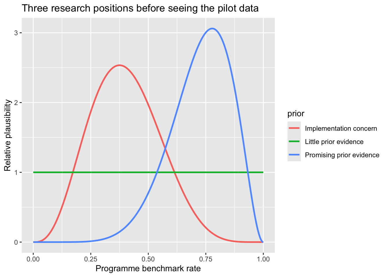
The three prior positions below represent three defensible research stories:

Little prior evidence: there is not enough prior evidence to favour any particular benchmark rate.
Implementation concern: earlier experience suggests the programme may struggle to reach a high benchmark rate.
Promising prior evidence: previous evidence gives some reason to expect a strong benchmark rate.

The curves below show these starting positions before the pilot data are used:

library(tidyverse)

theta_grid <- seq(0, 1, length.out = 1000)

prior_grid <- tibble(
  theta = theta_grid,
  `Little prior evidence` = dbeta(theta, 1, 1),
  `Implementation concern` = dbeta(theta, 4, 6),
  `Promising prior evidence` = dbeta(theta, 8, 3)
)

prior_grid |>
  pivot_longer(-theta, names_to = "prior", values_to = "density") |>
  ggplot(aes(theta, density, color = prior)) +
  geom_line(linewidth = 1) +
  labs(
    title = "Three research positions before seeing the pilot data",
    x = "Programme benchmark rate",
    y = "Relative plausibility"
  )

Use the panel below as a decision tool. Change the prior evidence, the pilot result, or the minimum useful rate to see how the scale-up judgement changes. It begins with the posterior view because the practical question is what is plausible after the pilot data have been seen.

Interactive beta-binomial update

Test the programme judgement

Adjust the pilot result, the minimum useful benchmark rate, and the prior evidence. The posterior shows what becomes plausible after the pilot is taken into account.

Pilot result Learners meeting benchmark Pilot learners Minimum useful rate

21 of 30 learners met the benchmark; useful rate = 0.60

Prior evidence

Little prior evidence Success weight Concern weight

Implementation concern Success weight Concern weight

Promising prior evidence Success weight Concern weight

Live distribution view

Posterior distributions after 21 of 30 learners reached the benchmark

Research position	Belief shown	Expected rate	95% credible range	P(rate > .60)	P(rate > .70)

Read the curves as three transparent research positions. The first says the researcher has little prior evidence and therefore lets the pilot carry most of the weight. The second says there are implementation concerns, perhaps because earlier roll-outs had low uptake or uneven teaching quality. The third says there is promising prior evidence, perhaps from a similar district or a previous cohort. None of these positions is right by definition. Each has to be justified from the education context.

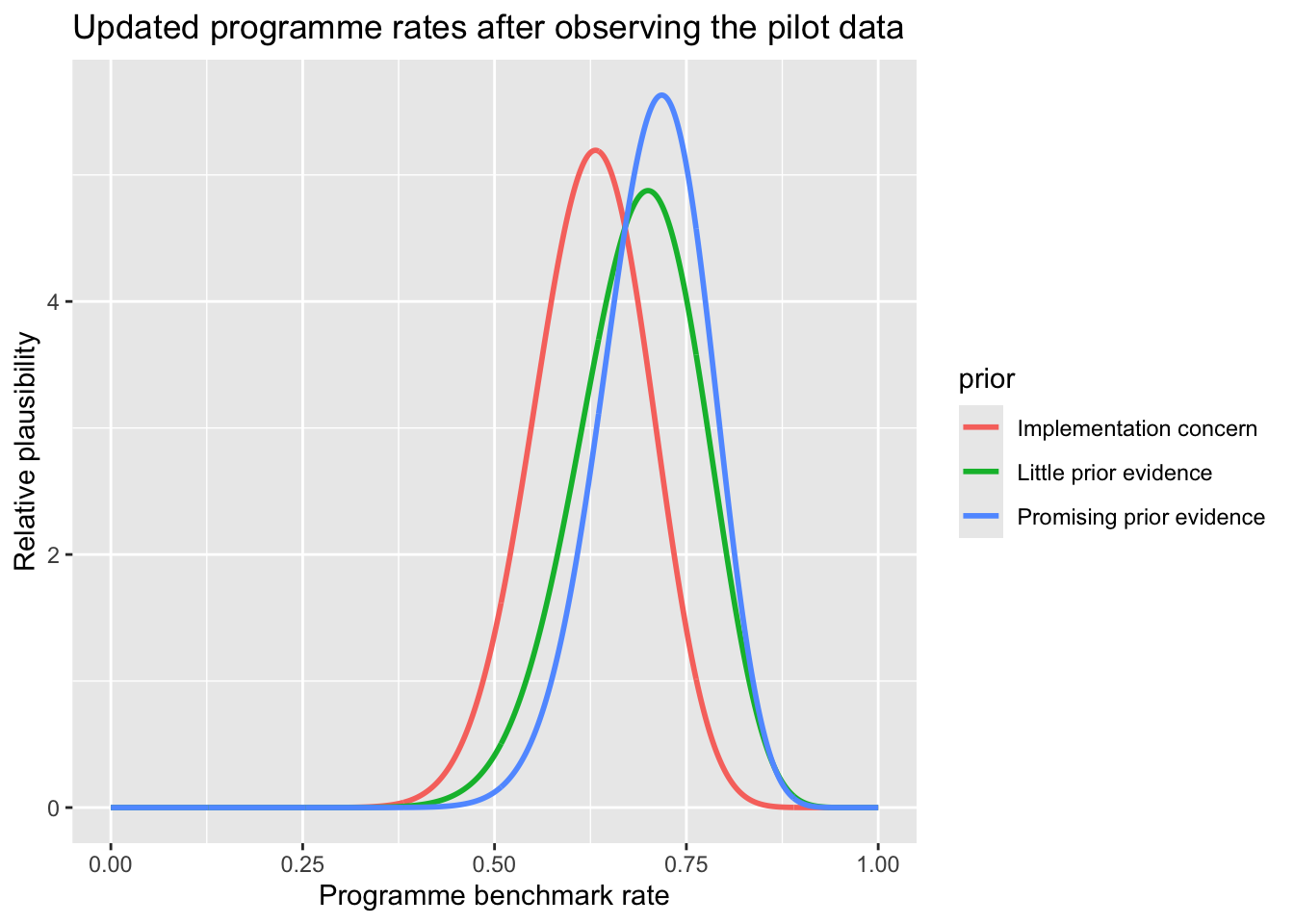
After observing 21 learners meeting the benchmark out of 30, the posterior for this simple model is:

theta | data ~ Beta(a + successes, b + failures)

failures <- n - successes

posterior_grid <- tibble(
  theta = theta_grid,
  `Little prior evidence` = dbeta(theta, 1 + successes, 1 + failures),
  `Implementation concern` = dbeta(theta, 4 + successes, 6 + failures),
  `Promising prior evidence` = dbeta(theta, 8 + successes, 3 + failures)
)

posterior_grid |>
  pivot_longer(-theta, names_to = "prior", values_to = "density") |>
  ggplot(aes(theta, density, color = prior)) +
  geom_line(linewidth = 1) +
  labs(
    title = "Updated programme rates after observing the pilot data",
    x = "Programme benchmark rate",
    y = "Relative plausibility"
  )

The three posterior distributions are more similar than the three starting positions. This is the point. The pilot data pull the research judgement towards the observed result: 21 of 30 learners reaching the benchmark. The promising-prior posterior sits slightly to the right because it began with stronger prior evidence for success. The implementation-concern posterior sits slightly to the left because it began with more prior caution. The little-prior-evidence posterior is closest to the raw pilot result because it lets the new data dominate.

This is the central logic of Bayesian updating. Prior evidence and new data both matter, but their relative weight depends on how informative each source is. With 30 learners, the prior positions still matter but they do not dominate. With only 3 learners, prior evidence would matter much more. With 300 learners, the pilot evidence would overwhelm these modest prior positions.

6 Posterior Summaries

summarise_beta <- function(a, b) {
  tibble(
    mean = a / (a + b),
    lower_95 = qbeta(0.025, a, b),
    upper_95 = qbeta(0.975, a, b),
    prob_above_60 = 1 - pbeta(0.60, a, b),
    prob_above_70 = 1 - pbeta(0.70, a, b)
  )
}

bind_rows(
  `Little prior evidence` = summarise_beta(1 + successes, 1 + failures),
  `Implementation concern` = summarise_beta(4 + successes, 6 + failures),
  `Promising prior evidence` = summarise_beta(8 + successes, 3 + failures),
  .id = "prior"
)

Where do the 95% and 86% come from?

For the reporting sentence below, we are using the row labelled “Little prior evidence”. That row starts with a neutral prior position and then updates it with the pilot result: 21 learners met the benchmark and 9 did not.

The 95% is used for the credible range. In this row, the middle 95% of the updated uncertainty runs from about 0.52 to 0.83. In words: under this model, the true programme success rate is plausibly somewhere between 52% and 83%.

The 86% answers a different question. It asks how much of the updated uncertainty lies above the 60% benchmark. In this row, about 86% of the posterior distribution is above 0.60.

Read this table as a set of possible reporting claims. The observed pilot result is 21 out of 30 learners, or 70%. Under little prior evidence, the posterior mean for the underlying programme success rate is close to 69%. The implementation-concern position pulls the posterior mean down because it gives more prior weight to learners not meeting the benchmark. The promising-prior position pulls it up because it gives more prior weight to success. The 95% credible intervals are wide because 30 learners is still a small pilot. The data are encouraging, but they do not pin the programme rate down tightly.

The probability columns matter most for applied reporting. prob_above_60 and prob_above_70 answer the question the district actually cares about: after seeing the pilot, how likely is it that the true programme rate exceeds a useful threshold? Under little prior evidence, the probability that the true programme rate exceeds 60% is roughly 0.86. This is separate from the credible interval. The credible interval describes where the true programme rate plausibly lies; the threshold probability describes how much of that uncertainty sits above 60%.

7 Interpretation

A practical Bayesian results statement using the little-prior-evidence row might read:

In the pilot, 21 of 30 learners met the reading benchmark, an observed success rate of 70%. Using the little-prior-evidence model, the posterior mean for the underlying programme success rate was 69%, with a 95% credible interval from 52% to 83%. The posterior probability that the true programme success rate exceeds the 60% benchmark was 86%.

What the frequentist analysis could not say directly

A frequentist analysis could report the observed success rate, provide a confidence interval, or test whether the pilot result is unusual under a threshold such as 60%. Those are useful summaries.

What it could not directly say is: there is an 86% probability that the true programme success rate is above 60%. That sentence is Bayesian because it treats the unknown success rate as the quantity about which uncertainty is being updated.

This statement is not merely saying that the result is statistically significant. It begins with the observed pilot rate, then reports the Bayesian estimate of the underlying programme rate, the 95% credible interval, and the probability that the rate clears the 60% decision threshold. The 86% is not a possible value of the programme rate, so it should not be compared with the endpoints of the credible interval. It is the probability mass above the 60% threshold. The credible interval is a probability statement about the unknown programme rate under the model. It is not the following frequentist statement:

If we repeated the sampling procedure many times, 95% of such intervals would contain the true parameter.

Why this matters for education reporting

A decision-maker does not only need to know whether the data are unusual under a null hypothesis.

They need to know how much uncertainty remains about the programme’s likely performance.

Bayesian inference returns that uncertainty directly, but it also requires the researcher to report the prior position and explain why it was reasonable.

Presenter caution

The Bayesian result gives us a clearer decision-facing statement, but it does not remove judgement. We still have to defend the prior, the model, the benchmark, the quality of the data, and the claim we are willing to make from a small pilot.

8 Exercise 1

Use the interactive panel to change the number of learners meeting the benchmark from 21 to 18 and then to 25.

For each case:

Record the probability that the programme rate exceeds 0.60 under each prior position.
Decide whether the programme would be described as promising, uncertain, or not yet convincing.
Write one sentence suitable for a district report.

9 Exercise 2

Change the minimum useful rate from 0.60 to 0.70.

Then answer:

Does the same pilot still look strong enough?
Which prior position changes the conclusion most?
What additional evidence would you want before recommending scale-up?

10 Exercise 3

Rewrite the following frequentist-style question as a Bayesian-style education research question:

Is the pass rate significantly above 60%?

Use this structure:

What is the probability that the programme ...

11 Takeaway

Bayesian analysis is useful here because it keeps the research question close to the education decision. Instead of stopping at whether the pilot result is statistically unusual, it asks how likely the programme is to meet a meaningful benchmark for future learners. The prior makes previous evidence and professional judgement visible. The likelihood lets the pilot data speak. The posterior combines them into a probability statement that can be reported, questioned, and defended. The rest of the workshop builds the discipline needed to choose those priors carefully, check the model, and write claims that remain honest about uncertainty.

--- title: "01 Bayesian Reasoning for Frequentist Researchers" subtitle: "From significance decisions to programme decisions under uncertainty" format: html: toc: true number-sections: true execute: warning: false message: false --- ```{=html} <nav class="module-route" aria-label="Notebook route"> <a class="active" href="01_bayesian_reasoning.html">01<br>Reasoning</a> <a href="02_priors.html">02<br>Priors</a> <a href="03_bayesian_regression.html">03<br>Regression</a> <a href="04_binary_and_ordinal_models.html">04<br>GLMs</a> <a href="05_hierarchical_models.html">05<br>Multilevel</a> <a href="06_model_checking.html">06<br>Checking</a> <a href="07_reporting.html">07<br>Reporting</a> </nav> ``` ## Learning Outcomes By the end of this session, you should be able to: 1. Translate an education research decision into a probability question. 2. Identify the unknown quantity a study is trying to learn about. 3. Treat prior evidence as a transparent research judgement rather than a hidden assumption. 4. Use a simple pilot study to update uncertainty about whether a programme is likely to meet a meaningful benchmark. ## The Programme Decision ```{=html} <style> .discussion-card { background: #fcf8ef; border: 1px solid rgba(13, 34, 64, 0.14); border-left: 4px solid #b8893c; border-radius: 6px; margin: 1rem 0 1.1rem; padding: 1rem 1.15rem; } .discussion-label { color: #b8893c; font-family: "JetBrains Mono", ui-monospace, monospace; font-size: 0.72rem; font-weight: 700; letter-spacing: 0.12em; margin: 0 0 0.4rem; text-transform: uppercase; } .discussion-question { color: #0d2240; font-family: "Newsreader", Georgia, serif; font-size: 1.35rem; line-height: 1.22; margin: 0; } .decision-question-card { background: #ffffff; border-color: rgba(184, 137, 60, 0.34); box-shadow: 0 14px 32px -30px rgba(13, 34, 64, 0.45); } .workshop-details { background: #ffffff; border: 1px solid rgba(13, 34, 64, 0.12); border-radius: 6px; margin: 0.35rem 0 1.3rem; padding: 0.75rem 1rem; } .workshop-details summary { color: #0d2240; cursor: pointer; font-weight: 700; } .judgement-map { display: grid; gap: 0.9rem; margin: 1.15rem 0 1.25rem; } .judgement-step { background: #ffffff; border: 1px solid rgba(13, 34, 64, 0.12); border-left: 4px solid #b8893c; border-radius: 6px; padding: 1rem 1.1rem; } .judgement-kicker { color: #b8893c; font-family: "JetBrains Mono", ui-monospace, monospace; font-size: 0.7rem; font-weight: 700; letter-spacing: 0.12em; margin: 0 0 0.35rem; text-transform: uppercase; } .judgement-title { color: #0d2240; font-family: "Newsreader", Georgia, serif; font-size: 1.25rem; line-height: 1.15; margin: 0 0 0.55rem; } .judgement-step p:last-child { margin-bottom: 0; } .judgement-step ul { margin: 0.55rem 0 0; padding-left: 1.15rem; } .judgement-step li { margin: 0.2rem 0; } .main-point-card { background: #fcf8ef; border: 1px solid rgba(184, 137, 60, 0.28); border-radius: 6px; margin: 1.15rem 0 1.35rem; padding: 1rem 1.15rem; } .main-point-card p:last-child { margin-bottom: 0; } @media (min-width: 900px) { .judgement-map { grid-template-columns: repeat(3, minmax(0, 1fr)); } } </style> ``` A district has piloted a reading support programme with 30 learners. At the end of the pilot, 21 learners reached the agreed reading proficiency benchmark. The district now has to decide what to do next. <div class="discussion-card"> <p class="discussion-label">Discuss first</p> <p class="discussion-question">Is this programme promising enough to continue, adapt, or scale?</p> </div> <details class="workshop-details"> <summary>Details</summary> That is not only a statistical question. It is a research judgement under uncertainty. The observed pilot result is encouraging, but 30 learners is a small group. The researcher has to decide what can be said responsibly about the larger population of similar learners who might receive the programme next year. </details> The headline figure is the observed pilot rate: ```{r} successes <- 21 n <- 30 successes / n ``` <div class="discussion-card"> <p class="discussion-label">Discuss first</p> <p class="discussion-question">What does the observed 70% tell us, and what does it not tell us?</p> </div> <details class="workshop-details"> <summary>Details</summary> Seventy per cent of the pilot learners reached the benchmark. That number is useful, but it is not the answer to the district's question. The district is not asking only what happened among these 30 learners. It is asking what is likely to happen if the programme is used with future learners in the same kind of setting. </details> <div class="discussion-card decision-question-card"> <p class="discussion-label">Bayesian decision question</p> <p class="discussion-question">What is the probability that the true benchmark success rate for this programme is above a minimum useful level, such as 60%?</p> </div> <div class="discussion-card"> <p class="discussion-label">Discuss first</p> <p class="discussion-question">What are the three parts of this question?</p> </div> <details class="workshop-details"> <summary>Details</summary> The question can be unpacked in three parts. The programme outcome is learners reaching the reading proficiency benchmark. The unknown quantity is the success rate we would expect among similar learners beyond this pilot. The decision line is 60%, the minimum rate being used here as a first marker of educational usefulness. </details> Bayesian analysis gives us a way to move from the pilot result to this kind of decision question. <details class="workshop-details"> <summary>Details</summary> Bayesian analysis helps organise that judgement. The prior records what was plausible before the pilot. The likelihood represents what the pilot data support. The posterior summarises what is now plausible after both sources of evidence have been considered. </details> ## The Shift Frequentist methods are useful, and they remain central to education research. They help researchers test clearly stated hypotheses, estimate uncertainty with confidence intervals, and avoid overclaiming from small studies. The shift in this workshop is not from "wrong" methods to "right" methods. It is from one kind of question to another. In a hypothesis test, the p-value is attached to a specific null hypothesis, often a hypothesis about a parameter. In many education studies, the usual null says that an effect, difference, association, or parameter is zero. For example, suppose an education researcher estimates a simple regression comparing learners who received a reading intervention with learners who did not: $$ Y_i = \beta_0 + \beta_1 D_i + \varepsilon_i. $$ Here, $Y_i$ is learner $i$'s reading outcome and $D_i$ indicates whether learner $i$ received the intervention. The coefficient $\beta_1$ is the estimated difference associated with the intervention. The usual null hypothesis is: $$ H_0 : \beta_1 = 0. $$ In words, the null says that the intervention coefficient is zero: no average difference in the reading outcome between the intervention and comparison groups, according to this model. A two-sided alternative would usually be written as: $$ H_1 : \beta_1 \neq 0. $$ The p-value then measures how unusual the observed data, or a result at least as extreme, would be if that zero-effect null model were true. ::: {.callout-note title="The key shift"} **Frequentist framing:** "If the programme's true success rate were 60%, how unusual would the eventual pilot result be once we observe how many learners reach the benchmark?" **Bayesian framing:** "After the pilot data are observed, what do we then believe about $\theta$, the programme's true success rate among similar learners?" ::: Before the intervention is run, the result is not known. If the planned pilot includes 30 learners, we can write the future number of learners who reach the benchmark as $X$. Once the pilot has been completed, the observed count will be written as $x_{\text{obs}}$, and the observed success rate will be: $$ \hat{\theta} = \frac{x_{\text{obs}}}{30}. $$ The district is not only interested in the eventual sample rate from those 30 learners. It wants to know what is plausible for the larger group of similar learners who might receive the programme in future. For the benchmark-rate question, we can write the unknown programme success rate as $\theta$. If 60% is the minimum useful rate, a frequentist one-sided test could be written as: $$ \begin{aligned} H_0 &: \theta = 0.60, \\ H_1 &: \theta > 0.60. \end{aligned} $$ For that test, the p-value is calculated after the pilot result is observed. If the observed count is $x_{\text{obs}}$, the p-value asks how unusual it would be to see $x_{\text{obs}}$ or more successes out of 30 learners if the true success rate were really 0.60: $$ p = \Pr\left(X \geq x_{\text{obs}} \mid X \sim \mathrm{Binomial}(30, 0.60)\right). $$ A frequentist analysis can test whether the eventual pilot result is compatible with a threshold such as 60%, or it can provide a confidence interval for the success rate after the data are collected. These are useful tools. However, they do not directly say, "There is a given probability that the true success rate is above 60%." A Bayesian analysis can express that uncertainty directly, conditional on the model and prior assumptions. ::: {.callout-warning title="Careful wording for education researchers"} - Do not say: "The p-value is the probability that the intervention does not work." - Rather say: "The p-value describes how unusual the observed data would be if the null model were true." - Do not say: "Bayesian analysis proves the programme works." - Rather say: "Bayesian analysis estimates how plausible different success rates are after considering the data and assumptions." ::: Once the pilot has been run, Bayesian analysis does not treat the observed sample rate as the final truth. It treats the observed result as evidence that updates uncertainty about the programme's true success rate. The posterior probability that the true success rate exceeds 60% provides a direct way of expressing how promising the programme appears, while still acknowledging uncertainty. ## Prior Evidence, New Data, Updated Judgement An education researcher rarely begins with no context. Before the pilot is run, there may already be evidence from earlier evaluations, teacher reports, implementation records, curriculum alignment, learner profiles, or experience with similar programmes. These things do not settle the question, but they shape what would count as a surprising or unsurprising result. Bayesian analysis gives that ordinary research judgement a clear structure. It asks three practical questions. <div class="judgement-map"> <section class="judgement-step"> <p class="judgement-kicker">Before the pilot</p> <p class="judgement-title">What seemed plausible?</p> <p>The district may have little previous evidence, reasons for caution because implementation was uneven, or good evidence from a similar setting.</p> <ul> <li>little previous evidence</li> <li>implementation concerns</li> <li>promising evidence from a similar context</li> </ul> </section> <section class="judgement-step"> <p class="judgement-kicker">Pilot evidence</p> <p class="judgement-title">What did the pilot add?</p> <p>If 21 out of 30 learners reached the benchmark, the result is encouraging. But the observed 70% is not the final answer. It is evidence about what might happen with similar learners in future.</p> </section> <section class="judgement-step"> <p class="judgement-kicker">Updated judgement</p> <p class="judgement-title">How should the judgement change?</p> <p>The updated judgement should speak directly to the education decision: how plausible is it that the programme would clear a meaningful benchmark, such as 60%, if used with similar learners?</p> </section> </div> <div class="main-point-card"> <p class="discussion-label">Main point</p> <p>Bayesian analysis is not asking education researchers to replace their research questions with statistical machinery. It asks them to make their starting assumptions visible, let the new data change those assumptions, and report the resulting uncertainty in a form that speaks directly to the programme decision.</p> </div> ## A Practical Updating Model For a benchmark outcome, each learner either reached the proficiency benchmark or did not. A simple model for this kind of outcome is: ```text successes ~ Binomial(n, theta) theta ~ Beta(a, b) ``` The first line says that the number of learners meeting the benchmark is modelled as a count out of `n` learners, governed by the unknown programme rate `theta`. The second line says that our prior uncertainty about `theta` is represented with a beta distribution. For this first example, the research interpretation matters more than the technical name. The two beta parameters, `a` and `b`, can be read as prior successes and prior failures. They are not literal extra learners secretly added to the pilot. They are a transparent way of expressing how much prior evidence the researcher is allowing to matter. The three prior positions below represent three defensible research stories: - **Little prior evidence**: there is not enough prior evidence to favour any particular benchmark rate. - **Implementation concern**: earlier experience suggests the programme may struggle to reach a high benchmark rate. - **Promising prior evidence**: previous evidence gives some reason to expect a strong benchmark rate. The curves below show these starting positions before the pilot data are used: ```{r} library(tidyverse) theta_grid <- seq(0, 1, length.out = 1000) prior_grid <- tibble( theta = theta_grid, `Little prior evidence` = dbeta(theta, 1, 1), `Implementation concern` = dbeta(theta, 4, 6), `Promising prior evidence` = dbeta(theta, 8, 3) ) prior_grid |> pivot_longer(-theta, names_to = "prior", values_to = "density") |> ggplot(aes(theta, density, color = prior)) + geom_line(linewidth = 1) + labs( title = "Three research positions before seeing the pilot data", x = "Programme benchmark rate", y = "Relative plausibility" ) ``` Use the panel below as a decision tool. Change the prior evidence, the pilot result, or the minimum useful rate to see how the scale-up judgement changes. It begins with the posterior view because the practical question is what is plausible after the pilot data have been seen. ```{=html} <div class="prior-lab" id="prior-beta-lab" data-view="posterior"> <div class="prior-lab-head"> <div> <p class="prior-lab-kicker">Interactive beta-binomial update</p> <h3>Test the programme judgement</h3> <p>Adjust the pilot result, the minimum useful benchmark rate, and the prior evidence. The posterior shows what becomes plausible after the pilot is taken into account.</p> </div> <div class="mode-toggle" role="group" aria-label="Distribution view"> <button type="button" data-view="prior">Prior</button> <button type="button" class="is-active" data-view="posterior">Posterior</button> </div> </div> <div class="prior-lab-controls"> <fieldset class="prior-lab-data"> <legend>Pilot result</legend> <label> <span>Learners meeting benchmark</span> <input type="number" min="0" step="1" value="21" data-control="successes"> </label> <label> <span>Pilot learners</span> <input type="number" min="1" step="1" value="30" data-control="trials"> </label> <label> <span>Minimum useful rate</span> <input type="number" min="0.05" max="0.95" step="0.05" value="0.60" data-control="threshold"> </label> <p data-data-note>21 of 30 learners met the benchmark; useful rate = 0.60</p> </fieldset> <fieldset class="prior-lab-priors"> <legend>Prior evidence</legend> <div class="prior-row prior-row-head" aria-hidden="true"> <span>Research position</span> <span>Success weight</span> <span>Concern weight</span> </div> <div class="prior-row"> <span><i class="prior-swatch weak"></i>Little prior evidence</span> <label><span>Success weight</span><input type="number" min="0.5" max="80" step="0.5" value="1" data-alpha="weak"></label> <label><span>Concern weight</span><input type="number" min="0.5" max="80" step="0.5" value="1" data-beta="weak"></label> </div> <div class="prior-row"> <span><i class="prior-swatch skeptical"></i>Implementation concern</span> <label><span>Success weight</span><input type="number" min="0.5" max="80" step="0.5" value="4" data-alpha="skeptical"></label> <label><span>Concern weight</span><input type="number" min="0.5" max="80" step="0.5" value="6" data-beta="skeptical"></label> </div> <div class="prior-row"> <span><i class="prior-swatch optimistic"></i>Promising prior evidence</span> <label><span>Success weight</span><input type="number" min="0.5" max="80" step="0.5" value="8" data-alpha="optimistic"></label> <label><span>Concern weight</span><input type="number" min="0.5" max="80" step="0.5" value="3" data-beta="optimistic"></label> </div> </fieldset> </div> <div class="prior-chart-panel"> <div> <p class="prior-chart-kicker">Live distribution view</p> <h4 data-live-title>Posterior distributions after 21 of 30 learners reached the benchmark</h4> </div> <svg class="prior-chart" viewBox="0 0 760 430" role="img" aria-label="Interactive beta prior and posterior density chart"></svg> </div> <div class="prior-summary-wrap"> <table class="prior-summary"> <thead> <tr> <th>Research position</th> <th>Belief shown</th> <th>Expected rate</th> <th>95% credible range</th> <th data-threshold-heading>P(rate > .60)</th> <th>P(rate > .70)</th> </tr> </thead> <tbody></tbody> </table> </div> </div> <script> (() => { const root = document.getElementById("prior-beta-lab"); if (!root) return; const priors = [ { key: "weak", label: "Little prior evidence", color: "#4f6fb3" }, { key: "skeptical", label: "Implementation concern", color: "#4f9f52" }, { key: "optimistic", label: "Promising prior evidence", color: "#d47767" } ]; const svg = root.querySelector(".prior-chart"); const tbody = root.querySelector(".prior-summary tbody"); const liveTitle = root.querySelector("[data-live-title]"); const dataNote = root.querySelector("[data-data-note]"); const thresholdHeading = root.querySelector("[data-threshold-heading]"); const viewButtons = root.querySelectorAll(".mode-toggle button"); const successInput = root.querySelector('[data-control="successes"]'); const trialsInput = root.querySelector('[data-control="trials"]'); const thresholdInput = root.querySelector('[data-control="threshold"]'); const chart = { width: 760, height: 430, left: 66, right: 30, top: 48, bottom: 64 }; chart.plotWidth = chart.width - chart.left - chart.right; chart.plotHeight = chart.height - chart.top - chart.bottom; const clamp = (value, min, max) => Math.min(Math.max(value, min), max); const fmtParam = (value) => Number.isInteger(value) ? String(value) : value.toFixed(1); const fmtNum = (value) => value.toFixed(2); const fmtRate = (value) => value.toFixed(2).replace(/^0/, ""); function numberFrom(input, fallback, { min = -Infinity, max = Infinity, integer = false } = {}) { let value = Number.parseFloat(input.value); if (!Number.isFinite(value)) value = fallback; value = clamp(value, min, max); if (integer) value = Math.round(value); input.value = String(value); return value; } function logGamma(z) { const p = [ 676.5203681218851, -1259.1392167224028, 771.32342877765313, -176.61502916214059, 12.507343278686905, -0.13857109526572012, 9.9843695780195716e-6, 1.5056327351493116e-7 ]; if (z < 0.5) { return Math.log(Math.PI) - Math.log(Math.sin(Math.PI * z)) - logGamma(1 - z); } z -= 1; let x = 0.99999999999980993; for (let i = 0; i < p.length; i += 1) x += p[i] / (z + i + 1); const t = z + p.length - 0.5; return 0.9189385332046727 + (z + 0.5) * Math.log(t) - t + Math.log(x); } function betaPdf(x, alpha, beta) { const logBeta = logGamma(alpha) + logGamma(beta) - logGamma(alpha + beta); return Math.exp((alpha - 1) * Math.log(x) + (beta - 1) * Math.log(1 - x) - logBeta); } function betaDistribution(alpha, beta) { const points = []; const steps = 520; const minX = 0.001; const maxX = 0.999; for (let i = 0; i < steps; i += 1) { const x = minX + (i / (steps - 1)) * (maxX - minX); points.push({ x, y: betaPdf(x, alpha, beta), cdf: 0 }); } let area = 0; for (let i = 1; i < points.length; i += 1) { area += 0.5 * (points[i - 1].y + points[i].y) * (points[i].x - points[i - 1].x); } let running = 0; for (let i = 1; i < points.length; i += 1) { running += 0.5 * (points[i - 1].y + points[i].y) * (points[i].x - points[i - 1].x); points[i].cdf = running / area; } return points; } function cdfAt(points, target) { if (target <= points[0].x) return 0; if (target >= points[points.length - 1].x) return 1; for (let i = 1; i < points.length; i += 1) { if (points[i].x >= target) { const left = points[i - 1]; const right = points[i]; const weight = (target - left.x) / (right.x - left.x); return left.cdf + weight * (right.cdf - left.cdf); } } return 1; } function quantile(points, probability) { for (let i = 1; i < points.length; i += 1) { if (points[i].cdf >= probability) { const left = points[i - 1]; const right = points[i]; const weight = (probability - left.cdf) / (right.cdf - left.cdf || 1); return left.x + weight * (right.x - left.x); } } return points[points.length - 1].x; } function niceMax(value) { if (value <= 1.5) return 1.5; if (value <= 4) return Math.ceil(value * 2) / 2; return Math.ceil(value); } function drawChart(rows, axisMax, sampleRate = null) { const xScale = (x) => chart.left + x * chart.plotWidth; const yScale = (y) => chart.top + chart.plotHeight - (y / axisMax) * chart.plotHeight; const xTicks = [0, 0.25, 0.5, 0.75, 1]; const yTicks = [0, axisMax / 2, axisMax]; const pathFor = (points) => points .map((point, index) => `${index === 0 ? "M" : "L"} ${xScale(point.x).toFixed(2)} ${yScale(point.y).toFixed(2)}`) .join(" "); let html = ` <rect class="prior-chart-bg" x="${chart.left}" y="${chart.top}" width="${chart.plotWidth}" height="${chart.plotHeight}"></rect> `; xTicks.forEach((tick) => { const x = xScale(tick); html += ` <line class="prior-chart-grid" x1="${x}" x2="${x}" y1="${chart.top}" y2="${chart.top + chart.plotHeight}"></line> <text class="prior-chart-tick" x="${x}" y="${chart.top + chart.plotHeight + 26}" text-anchor="middle">${tick.toFixed(2)}</text> `; }); yTicks.forEach((tick) => { const y = yScale(tick); html += ` <line class="prior-chart-grid" x1="${chart.left}" x2="${chart.left + chart.plotWidth}" y1="${y}" y2="${y}"></line> <text class="prior-chart-tick" x="${chart.left - 14}" y="${y + 4}" text-anchor="end">${tick < 10 ? tick.toFixed(1) : tick.toFixed(0)}</text> `; }); rows.forEach((row) => { html += `<path class="prior-chart-line" d="${pathFor(row.points)}" stroke="${row.color}"></path>`; }); if (sampleRate !== null) { const rate = clamp(sampleRate, 0, 1); const sampleX = xScale(rate); const anchor = rate > 0.72 ? "end" : "start"; const labelX = anchor === "end" ? sampleX - 8 : sampleX + 8; html += ` <line class="prior-sample-line" x1="${sampleX}" x2="${sampleX}" y1="${chart.top}" y2="${chart.top + chart.plotHeight}"></line> <text class="prior-sample-label" x="${labelX}" y="${chart.top + 18}" text-anchor="${anchor}">Pilot rate ${rate.toFixed(2)}</text> `; } html += ` <line class="prior-chart-axis" x1="${chart.left}" x2="${chart.left + chart.plotWidth}" y1="${chart.top + chart.plotHeight}" y2="${chart.top + chart.plotHeight}"></line> <line class="prior-chart-axis" x1="${chart.left}" x2="${chart.left}" y1="${chart.top}" y2="${chart.top + chart.plotHeight}"></line> <text class="prior-chart-label" x="${chart.left + chart.plotWidth / 2}" y="${chart.height - 14}" text-anchor="middle">Programme benchmark rate</text> <text class="prior-chart-label" transform="translate(18 ${chart.top + chart.plotHeight / 2}) rotate(-90)" text-anchor="middle">Relative plausibility</text> `; rows.forEach((row, index) => { const x = chart.left + index * 148; html += ` <line class="prior-chart-legend-line" x1="${x}" x2="${x + 28}" y1="22" y2="22" stroke="${row.color}"></line> <text class="prior-chart-legend" x="${x + 36}" y="26">${row.label}</text> `; }); svg.innerHTML = html; } function setView(view) { root.dataset.view = view; } function update(source = null) { if (source?.dataset.control) { setView("posterior"); } const trials = numberFrom(trialsInput, 30, { min: 1, max: 500, integer: true }); const successes = numberFrom(successInput, 21, { min: 0, max: trials, integer: true }); const threshold = numberFrom(thresholdInput, 0.6, { min: 0.05, max: 0.95 }); const failures = trials - successes; const view = root.dataset.view || "prior"; viewButtons.forEach((button) => { button.classList.toggle("is-active", button.dataset.view === view); }); dataNote.textContent = `${successes} of ${trials} learners met the benchmark; useful rate = ${threshold.toFixed(2)}`; thresholdHeading.textContent = `P(rate > ${fmtRate(threshold)})`; liveTitle.textContent = view === "posterior" ? `Posterior distributions after ${successes} of ${trials} learners reached the benchmark` : "Prior beliefs before seeing the pilot data"; const rows = priors.map((prior) => { const alphaInput = root.querySelector(`[data-alpha="${prior.key}"]`); const betaInput = root.querySelector(`[data-beta="${prior.key}"]`); const priorAlpha = numberFrom(alphaInput, 1, { min: 0.5, max: 80 }); const priorBeta = numberFrom(betaInput, 1, { min: 0.5, max: 80 }); const alpha = priorAlpha + (view === "posterior" ? successes : 0); const beta = priorBeta + (view === "posterior" ? failures : 0); const points = betaDistribution(alpha, beta); return { ...prior, alpha, beta, points, mean: alpha / (alpha + beta), lower: quantile(points, 0.025), upper: quantile(points, 0.975), probThreshold: 1 - cdfAt(points, threshold), prob70: 1 - cdfAt(points, 0.7) }; }); const axisMax = niceMax(Math.max(...rows.flatMap((row) => row.points.map((point) => point.y))) * 1.08); drawChart(rows, axisMax, view === "posterior" ? successes / trials : null); tbody.innerHTML = rows.map((row) => ` <tr> <td><span class="prior-table-swatch" style="background:${row.color}"></span>${row.label}</td> <td>Beta(${fmtParam(row.alpha)}, ${fmtParam(row.beta)})</td> <td>${fmtNum(row.mean)}</td> <td>${fmtNum(row.lower)} to ${fmtNum(row.upper)}</td> <td>${fmtNum(row.probThreshold)}</td> <td>${fmtNum(row.prob70)}</td> </tr> `).join(""); } root.querySelectorAll("input").forEach((input) => { input.addEventListener("input", () => update(input)); input.addEventListener("change", () => update(input)); }); viewButtons.forEach((button) => { button.addEventListener("click", () => { setView(button.dataset.view); update(); }); }); update(); })(); </script> ``` Read the curves as three transparent research positions. The first says the researcher has little prior evidence and therefore lets the pilot carry most of the weight. The second says there are implementation concerns, perhaps because earlier roll-outs had low uptake or uneven teaching quality. The third says there is promising prior evidence, perhaps from a similar district or a previous cohort. None of these positions is right by definition. Each has to be justified from the education context. After observing 21 learners meeting the benchmark out of 30, the posterior for this simple model is: ```text theta | data ~ Beta(a + successes, b + failures) ``` ```{r} failures <- n - successes posterior_grid <- tibble( theta = theta_grid, `Little prior evidence` = dbeta(theta, 1 + successes, 1 + failures), `Implementation concern` = dbeta(theta, 4 + successes, 6 + failures), `Promising prior evidence` = dbeta(theta, 8 + successes, 3 + failures) ) posterior_grid |> pivot_longer(-theta, names_to = "prior", values_to = "density") |> ggplot(aes(theta, density, color = prior)) + geom_line(linewidth = 1) + labs( title = "Updated programme rates after observing the pilot data", x = "Programme benchmark rate", y = "Relative plausibility" ) ``` The three posterior distributions are more similar than the three starting positions. This is the point. The pilot data pull the research judgement towards the observed result: 21 of 30 learners reaching the benchmark. The promising-prior posterior sits slightly to the right because it began with stronger prior evidence for success. The implementation-concern posterior sits slightly to the left because it began with more prior caution. The little-prior-evidence posterior is closest to the raw pilot result because it lets the new data dominate. This is the central logic of Bayesian updating. Prior evidence and new data both matter, but their relative weight depends on how informative each source is. With 30 learners, the prior positions still matter but they do not dominate. With only 3 learners, prior evidence would matter much more. With 300 learners, the pilot evidence would overwhelm these modest prior positions. ## Posterior Summaries ```{r} summarise_beta <- function(a, b) { tibble( mean = a / (a + b), lower_95 = qbeta(0.025, a, b), upper_95 = qbeta(0.975, a, b), prob_above_60 = 1 - pbeta(0.60, a, b), prob_above_70 = 1 - pbeta(0.70, a, b) ) } bind_rows( `Little prior evidence` = summarise_beta(1 + successes, 1 + failures), `Implementation concern` = summarise_beta(4 + successes, 6 + failures), `Promising prior evidence` = summarise_beta(8 + successes, 3 + failures), .id = "prior" ) ``` ::: {.callout-note title="Where do the 95% and 86% come from?"} For the reporting sentence below, we are using the row labelled "Little prior evidence". That row starts with a neutral prior position and then updates it with the pilot result: 21 learners met the benchmark and 9 did not. The 95% is used for the credible range. In this row, the middle 95% of the updated uncertainty runs from about 0.52 to 0.83. In words: under this model, the true programme success rate is plausibly somewhere between 52% and 83%. The 86% answers a different question. It asks how much of the updated uncertainty lies above the 60% benchmark. In this row, about 86% of the posterior distribution is above 0.60. ::: Read this table as a set of possible reporting claims. The observed pilot result is 21 out of 30 learners, or 70%. Under little prior evidence, the posterior mean for the underlying programme success rate is close to 69%. The implementation-concern position pulls the posterior mean down because it gives more prior weight to learners not meeting the benchmark. The promising-prior position pulls it up because it gives more prior weight to success. The 95% credible intervals are wide because 30 learners is still a small pilot. The data are encouraging, but they do not pin the programme rate down tightly. The probability columns matter most for applied reporting. `prob_above_60` and `prob_above_70` answer the question the district actually cares about: after seeing the pilot, how likely is it that the true programme rate exceeds a useful threshold? Under little prior evidence, the probability that the true programme rate exceeds 60% is roughly 0.86. This is separate from the credible interval. The credible interval describes where the true programme rate plausibly lies; the threshold probability describes how much of that uncertainty sits above 60%. ## Interpretation A practical Bayesian results statement using the little-prior-evidence row might read: > In the pilot, 21 of 30 learners met the reading benchmark, an observed success rate of 70%. Using the little-prior-evidence model, the posterior mean for the underlying programme success rate was 69%, with a 95% credible interval from 52% to 83%. The posterior probability that the true programme success rate exceeds the 60% benchmark was 86%. ::: {.callout-note title="What the frequentist analysis could not say directly"} A frequentist analysis could report the observed success rate, provide a confidence interval, or test whether the pilot result is unusual under a threshold such as 60%. Those are useful summaries. What it could not directly say is: there is an 86% probability that the true programme success rate is above 60%. That sentence is Bayesian because it treats the unknown success rate as the quantity about which uncertainty is being updated. ::: This statement is not merely saying that the result is statistically significant. It begins with the observed pilot rate, then reports the Bayesian estimate of the underlying programme rate, the 95% credible interval, and the probability that the rate clears the 60% decision threshold. The 86% is not a possible value of the programme rate, so it should not be compared with the endpoints of the credible interval. It is the probability mass above the 60% threshold. The credible interval is a probability statement about the unknown programme rate under the model. It is not the following frequentist statement: > If we repeated the sampling procedure many times, 95% of such intervals would contain the true parameter. ::: {.callout-tip title="Why this matters for education reporting"} A decision-maker does not only need to know whether the data are unusual under a null hypothesis. They need to know how much uncertainty remains about the programme's likely performance. Bayesian inference returns that uncertainty directly, but it also requires the researcher to report the prior position and explain why it was reasonable. ::: ::: {.callout-warning title="Presenter caution"} The Bayesian result gives us a clearer decision-facing statement, but it does not remove judgement. We still have to defend the prior, the model, the benchmark, the quality of the data, and the claim we are willing to make from a small pilot. ::: ## Exercise 1 Use the interactive panel to change the number of learners meeting the benchmark from 21 to 18 and then to 25. For each case: 1. Record the probability that the programme rate exceeds 0.60 under each prior position. 2. Decide whether the programme would be described as promising, uncertain, or not yet convincing. 3. Write one sentence suitable for a district report. ## Exercise 2 Change the minimum useful rate from 0.60 to 0.70. Then answer: 1. Does the same pilot still look strong enough? 2. Which prior position changes the conclusion most? 3. What additional evidence would you want before recommending scale-up? ## Exercise 3 Rewrite the following frequentist-style question as a Bayesian-style education research question: > Is the pass rate significantly above 60%? Use this structure: ```text What is the probability that the programme ... ``` ## Takeaway Bayesian analysis is useful here because it keeps the research question close to the education decision. Instead of stopping at whether the pilot result is statistically unusual, it asks how likely the programme is to meet a meaningful benchmark for future learners. The prior makes previous evidence and professional judgement visible. The likelihood lets the pilot data speak. The posterior combines them into a probability statement that can be reported, questioned, and defended. The rest of the workshop builds the discipline needed to choose those priors carefully, check the model, and write claims that remain honest about uncertainty. ```{=html} <nav class="module-nav" aria-label="Module navigation"> <a href="../index.html">← Workshop Home</a> <a href="02_priors.html">Next: Priors →</a> </nav> ```