library(readr)
library(ggplot2)

education <- read_csv("data/education_intervention.csv")02 Priors and Prior Predictive Checks
Making assumptions explicit and testable
1 Learning Outcomes
By the end of this module, participants should be able to:
- Explain a prior as a transparent research judgement made before the new evidence is used.
- Translate education expectations into plausible ranges on the outcome scale.
- Check whether those expectations would generate believable learner outcomes.
- Write a defensible prior justification that another researcher can inspect and challenge.
2 The Education Question
A district is evaluating an education intervention intended to improve endline test scores. Before the new analysis is used to make claims about the programme, the researcher has to decide what kinds of programme effects would be believable.
Research judgement
Before looking at the new programme evidence, what improvement in learner scores would be plausible, surprising, or too large to believe?
That question is the entry point to priors. A prior is not a decorative statistical object. It is the researcher’s stated position about what was plausible before the new data were allowed to change that position.
Details
Education researchers already make this kind of judgement. They decide whether a reported effect is educationally meaningful, whether an implementation setting is comparable to earlier studies, and whether a claimed gain is credible on the score scale being used. Bayesian analysis asks us to write that judgement down, check it, and make it available for criticism.
3 The Score Scale
The main dataset studies whether an education intervention improves endline test scores.
3.1 Dataset Overview
Before choosing priors, we only need enough information to understand the scale of the variables. The main variables are:
| Variable | How to read it |
|---|---|
endline_score |
The learner’s score at the end of the study, measured on a 0-100 scale. Higher values mean stronger performance. |
intervention |
Whether the learner received the programme. A value of 1 means treated; 0 means comparison. |
baseline_score |
The learner’s score before the intervention period. |
ses_index |
A standardised socioeconomic-status measure. A value of 0 is roughly average SES in this sample; 1 is about one standard deviation above average; -1 is about one standard deviation below average. |
attendance_rate |
Learner attendance percentage during the study period. |
Because endline_score is measured in score points, the prior expectations must also make sense in score points. A prior that treats a 200-point improvement as plausible is not being open-minded. It is ignoring the measurement scale.
Here, SES means socioeconomic status. The ses_index variable is a constructed background measure, not a test score. Because it has been standardised, a value of 0 represents roughly average SES in this sample, a value of 1 represents about one standard deviation above average, and a value of -1 represents about one standard deviation below average. In the regression, the SES coefficient is therefore read as the expected difference in endline score associated with a one-standard-deviation higher SES index, after accounting for intervention status and baseline score.
A short R summary is enough for this purpose:
summary(education[c(
  "endline_score",
  "baseline_score",
  "ses_index",
  "attendance_rate"
)])
endline_score baseline_score ses_index attendance_rate
Min. : 34.72 Min. :25.65 Min. :-2.20000 Min. : 62.19
1st Qu.: 61.71 1st Qu.:51.51 1st Qu.:-0.58800 1st Qu.: 79.34
Median : 70.47 Median :58.63 Median : 0.01700 Median : 84.39
Mean : 70.40 Mean :58.03 Mean :-0.01687 Mean : 84.32
3rd Qu.: 78.38 3rd Qu.:65.84 3rd Qu.: 0.55800 3rd Qu.: 89.42
Max. :100.00 Max. :93.74 Max. : 2.20000 Max. :100.00 table(education$intervention)
  0   1
129 132
3.2 Treatment Balance
In an applied study, the first question is whether treated and control groups are comparable on covariates before the intervention. Imbalance does not invalidate a model, but it does change which priors and adjustments make sense.
aggregate(
  cbind(baseline_score, ses_index, attendance_rate) ~ intervention,
  data = education,
  FUN = mean
)
3.3 Outcome Scale and Plausible Effect Sizes
The distribution of endline scores helps us speak in the same units as the education decision:
ggplot(education, aes(x = endline_score)) +
  geom_histogram(binwidth = 2) +
  geom_vline(xintercept = mean(education$endline_score), linetype = "dashed") +
  labs(
    title = "Endline score distribution",
    x = "Endline score (0-100)",
    y = "Count"
  )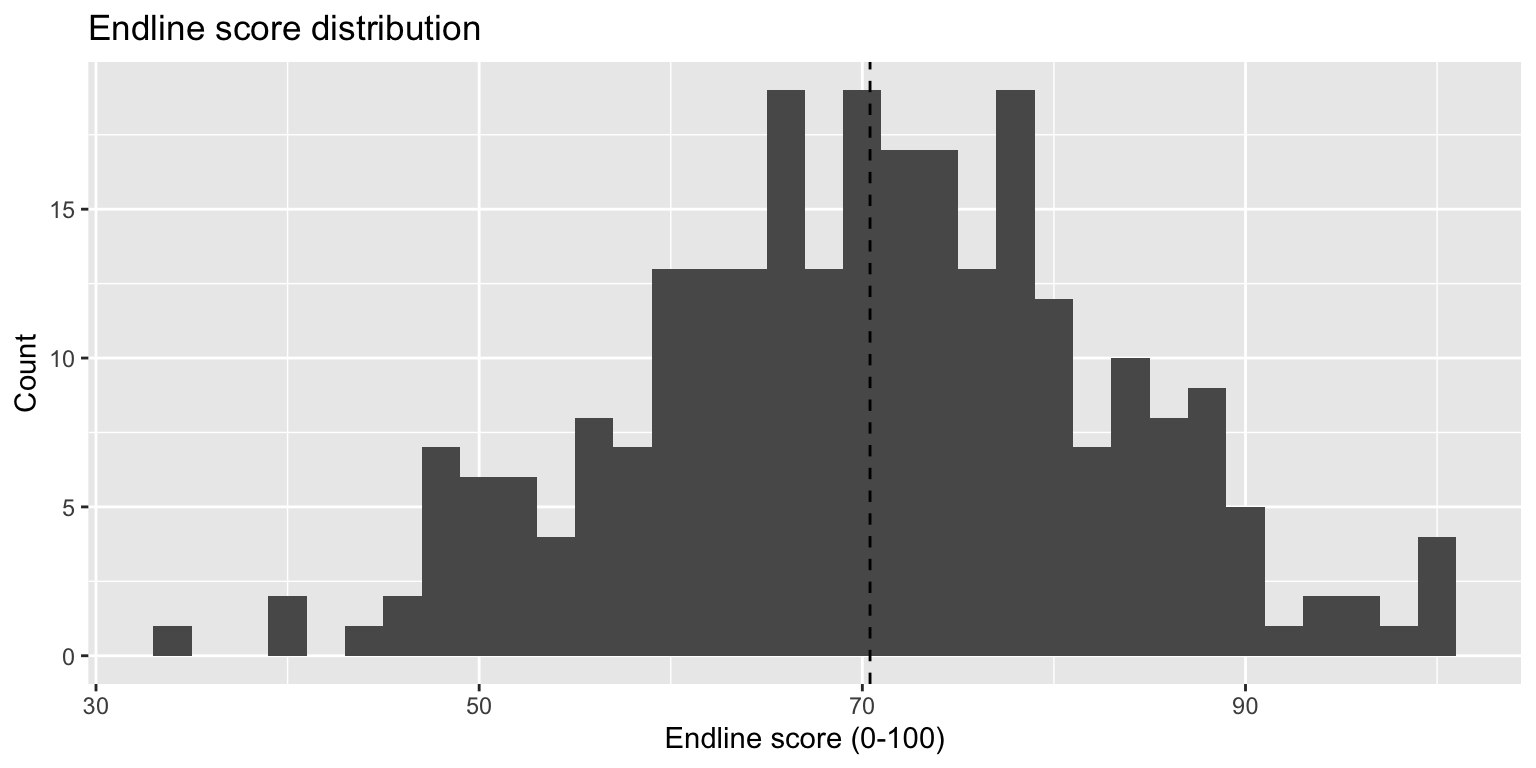
A substantively meaningful improvement on this outcome might be 3 points or more. That does not mean 3 points is automatically large enough for every policy decision. It simply gives the workshop a practical threshold: a gain below this may be too small to matter educationally, while a gain well above this would be increasingly noteworthy.
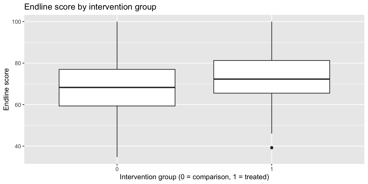
The group comparison below is descriptive. It helps us see what the dataset contains, but it should not be used to invent the prior for this same analysis.
ggplot(education, aes(x = factor(intervention), y = endline_score)) +
  geom_boxplot() +
  labs(
    title = "Endline score by intervention group",
    x = "Intervention group (0 = comparison, 1 = treated)",
    y = "Endline score"
  )
Discuss first
On a 0-100 reading score, what programme gains would you describe as negligible, useful, large, or implausibly large?
Details
The exact cut-offs depend on the assessment, the grade level, the cost of the intervention, and the decision being made. The important point is that the prior should live on this substantive scale. If an education researcher cannot explain what a 3-point, 10-point, or 20-point gain would mean, the prior cannot be defended.
4 Three Starting Positions
For the intervention effect, the prior answers a practical question:
Before using the new outcome data, what range of programme effects would we regard as believable?
The workshop uses three starting positions. They are not tricks, and none of them is automatically correct. Each one represents a different research judgement.
Little prior evidence
Keep the starting position wide
There is not much previous evidence from similar settings. Very large effects are still treated as unlikely, but the analysis begins with a wide range of possible gains and losses.
Implementation caution
Expect modest effects
Earlier implementation has been uneven, or similar interventions have produced small effects. The prior allows improvement, but it treats large gains as less plausible before seeing the new data.
Promising previous evidence
Start with a positive expectation
A closely related study or pilot suggests a meaningful improvement. The prior begins with a positive expectation, but still allows the new data to weaken that expectation.
The same three positions can be written as statistical priors on the intervention effect. Read the notation as a compact way of writing the research judgement:
| Starting position | Statistical form | Plain-language reading |
|---|---|---|
| Little prior evidence | Normal(0, 10) | The starting expectation is no average difference, but effects from roughly -20 to +20 score points are still treated as possible. |
| Implementation caution | Normal(0, 3) | The starting expectation is no average difference, and most believable effects fall between roughly -6 and +6 score points. |
| Promising previous evidence | Normal(4, 3) | Previous evidence points to an improvement of about 4 score points, but smaller, larger, or even negative effects remain possible. |
The zero in Normal(0, 10) or Normal(0, 3) does not mean the researcher believes the programme has no effect. It means the researcher is not building in a positive effect before the new evidence is considered. The spread of the prior says how wide the range of believable effects is.
Presenter line
The prior is not the conclusion. It is the starting position we are willing to defend before the new evidence is allowed to move us.
5 Checking the Starting Positions
The common worry is that priors allow the researcher to smuggle in a preferred answer. The practical response is to check what the prior implies before fitting the model.
The check asks:
If this starting position were used, what kinds of programme effects would it make believable?
The short code below plots the three starting positions on the score-point scale.
curve(
  dnorm(x, mean = 0, sd = 10),
  from = -30,
  to = 30,
  lwd = 2,
  col = "steelblue",
  xlab = "Intervention effect in score points",
  ylab = "Density"
)

curve(
  dnorm(x, mean = 0, sd = 3),
  add = TRUE,
  lwd = 2,
  col = "darkgreen"
)

curve(
  dnorm(x, mean = 4, sd = 3),
  add = TRUE,
  lwd = 2,
  col = "firebrick"
)

abline(v = 3, lty = 2)

legend(
  "topright",
  legend = c("Little prior evidence", "Implementation caution", "Promising previous evidence"),
  col = c("steelblue", "darkgreen", "firebrick"),
  lwd = 2,
  bty = "n"
)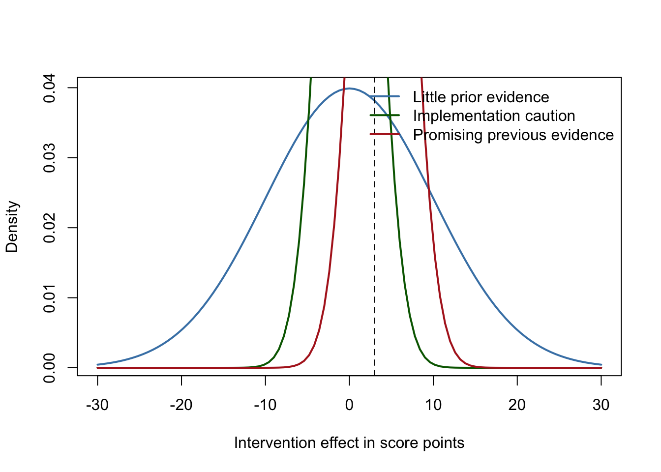
The dashed vertical line marks the 3-point threshold. The wide starting position treats a 3-point effect as believable but not specially favoured. The cautious starting position keeps most of its mass near zero and would need stronger evidence before accepting a large gain. The evidence-informed starting position places more weight above 3 points, so it needs a clear explanation of where that previous evidence came from.
Discuss first
Which starting position would be easiest to defend to a sceptical education researcher, and what evidence would justify it?
Details
The answer depends on the setting. With little previous evidence, the wide prior is easier to defend than a positive prior. If previous implementation was uneven, the cautious prior may be more honest. If a closely related evaluation already found a 4-point gain, the evidence-informed prior may be defensible, but the source of that evidence must be named.
6 Checking the Whole Model in brms
A fuller check asks whether the whole model, using the prior alone, can generate believable learner scores. This is useful because a prior may sound reasonable for one coefficient but still create impossible outcomes when combined with the intercept, baseline score, SES, and residual variation.
The code below is marked eval: false because it requires a working Stan installation. The pattern is the important part: define the starting assumptions, ask the model to simulate from those assumptions only, and then inspect whether the simulated scores look plausible.
library(brms)

prior_model <- brm(
  endline_score ~ intervention + baseline_score + ses_index,
  data = education,
  family = gaussian(),
  prior = c(
    prior(normal(60, 15), class = "Intercept"),
    prior(normal(0, 10), class = "b", coef = "intervention"),
    prior(normal(0.6, 0.2), class = "b", coef = "baseline_score"),
    prior(normal(0, 4), class = "b", coef = "ses_index"),
    prior(exponential(1), class = "sigma")
  ),
  sample_prior = "only",
  backend = "cmdstanr",
  chains = 4,
  cores = 4,
  iter = 1000
)

pp_check(prior_model, ndraws = 50)
The class labels in the code tell brms which part of the regression the prior belongs to. Intercept is the expected score for the reference case. b means regression coefficient, such as the intervention effect or the baseline-score adjustment. sigma is the remaining spread in scores after the model has used the predictors.
Read the check in education terms: if the model repeatedly simulates scores below 0, above 100, or group differences that would be impossible to defend in this setting, the priors need to be revised before the analysis is fitted.
7 Prior Justification Table
For a reportable analysis, each prior decision should be paired with a justification and a check. The table below is an audit trail: it shows what the assumption means, why it is reasonable, and what would make it questionable.
| Model quantity | Prior | Education reading | What to check |
|---|---|---|---|
| Intercept | Normal(60, 15) | Expected endline scores should usually sit inside the 0-100 scale. | Does it generate many impossible scores? |
| Intervention | Normal(0, 10) | With little prior evidence, allow a wide range of gains and losses but rule out absurd effects. | Does it imply programme gains too large to defend? |
| Baseline score | Normal(0.6, 0.2) | Learners who start higher are expected to end higher, but baseline should not mechanically determine the endline score. | Does it force too strong a baseline-endline relationship? |
| SES index | Normal(0, 4) | A one-standard-deviation higher SES index may be associated with higher or lower endline scores after adjustment, but the gap should remain modest. | Does it imply implausibly large score differences between learners from different socioeconomic backgrounds? |
| Residual spread | Exponential(1) | Learners will still differ after intervention status, baseline score, and SES are considered. | Is the remaining variation unrealistically small or large? |
8 Exercise
Choose one education intervention you know. Then define three possible starting positions for its effect on a 0-100 outcome scale:
- Little prior evidence.
- Implementation caution.
- Promising previous evidence.
For each starting position:
- State the range of score-point effects it treats as plausible.
- Say what evidence would justify that range.
- Say what would make that starting position inappropriate.
9 Reporting Priors
A methods-reporting version:
The intervention coefficient was assigned a weakly informative Normal(0, 10) prior on the score-point scale. This prior centres the effect at no difference while allowing effects large enough to cover plausible educational impacts. We checked the prior predictive distribution to ensure it did not place substantial probability on impossible or substantively implausible outcome values.
A more education-facing version:
Before analysing the programme effect, we used a deliberately wide starting position. It did not assume the intervention would work, but it allowed for educationally meaningful gains or losses while ruling out effects too large to be credible on the 0-100 score scale. We checked that this starting position generated believable learner scores before fitting the model.
10 Takeaway
Priors are not a request for education researchers to become more technical. They are a way of making a familiar research judgement visible: what did we think was plausible before this dataset changed our mind? The notation matters, but it comes second. First comes the education question, the outcome scale, the meaningful threshold, and the evidence that makes a starting position defensible.