workflow <- read.csv("data/frequentist_workflow_education.csv")Frequentist Workflow for Social Science Research
Validation, analysis, and reporting for education researchers
Frequentist workflow
This page is for researchers who need results they can understand, defend, and write into a paper.
It assumes participants already know the basic idea of p-values. The focus is not to teach a catalogue of tests. The focus is to move from an education research question to a result, and from the result to a careful reporting sentence.
1 Running Study
Education study
A district has evaluated a reading support programme. The dataset contains learners’ baseline reading scores, endline reading scores, school context, attendance, SES, four engagement items, intervention status, and whether each learner reached the reading benchmark.
The paper is not trying to show every possible test. It is trying to build a defensible results section around connected questions:
- Are the data and measures ready to analyse?
- Can the engagement items be treated as one scale?
- Do learners who received the programme perform better?
- Do results differ across school contexts?
- Is engagement related to reading achievement?
- Does the programme still matter after accounting for baseline reading and learner background?
2 The Research Workflow
The order matters. A defensible paper does not begin with a test. It begins with the research question, the quality of the measures, and the structure of the data.
Question. What is the paper trying to claim: a difference, association, prediction, programme effect, or measurement result?
Validation. Are the variables coded correctly, are missing values visible, and does the scale measure one coherent construct?
Description. What do the raw results show before any formal model is fitted?
Analysis. Which short analysis answers the research question without adding unnecessary machinery?
Checking. Are the assumptions reasonable enough for the claim being made?
Reporting. What sentence can be written honestly in a social science paper?
From this point on, every analysis uses the same dataset. That is deliberate: participants should see how one study can move from validation to description, analysis, and reporting without changing examples every few minutes.
3 Data Validation Before Analysis
Question
Does the dataset contain what the paper says it contains?
This step is not administrative. It protects the paper from reporting results based on miscoded groups, missing outcomes, impossible values, or variables that do not match the research question. In participants’ own papers, this is where they confirm that the analysis file is genuinely ready to support the claims they want to make.
names(workflow) [1] "learner_id" "school_id" "school_context"
[4] "intervention" "gender" "ses_index"
[7] "baseline_reading" "attendance_rate" "engage_attention"
[10] "engage_participation" "engage_homework" "engage_persistence"
[13] "endline_reading" "met_benchmark" summary(workflow) learner_id school_id school_context intervention
Length:312 Length:312 Length:312 Min. :0.0000
Class :character Class :character Class :character 1st Qu.:0.0000
Mode :character Mode :character Mode :character Median :0.0000
Mean :0.4904
3rd Qu.:1.0000
Max. :1.0000
gender ses_index baseline_reading attendance_rate
Length:312 Min. :-1.9650 Min. :25.00 Min. :62.31
Class :character 1st Qu.:-0.3860 1st Qu.:49.75 1st Qu.:75.61
Mode :character Median : 0.1395 Median :57.61 Median :82.36
Mean : 0.1638 Mean :57.57 Mean :82.22
3rd Qu.: 0.7880 3rd Qu.:65.39 3rd Qu.:88.88
Max. : 2.5000 Max. :88.18 Max. :99.00
engage_attention engage_participation engage_homework engage_persistence
Min. :1.000 Min. :1.000 Min. :1.000 Min. :1.000
1st Qu.:2.000 1st Qu.:2.000 1st Qu.:2.000 1st Qu.:2.000
Median :3.000 Median :3.000 Median :3.000 Median :3.000
Mean :3.141 Mean :3.317 Mean :3.045 Mean :3.237
3rd Qu.:4.000 3rd Qu.:4.000 3rd Qu.:4.000 3rd Qu.:4.000
Max. :5.000 Max. :5.000 Max. :5.000 Max. :5.000
endline_reading met_benchmark
Min. : 29.37 Min. :0.0000
1st Qu.: 59.69 1st Qu.:0.0000
Median : 68.60 Median :1.0000
Mean : 68.96 Mean :0.7404
3rd Qu.: 79.58 3rd Qu.:1.0000
Max. :100.00 Max. :1.0000 colSums(is.na(workflow)) learner_id school_id school_context
0 0 0
intervention gender ses_index
0 0 0
baseline_reading attendance_rate engage_attention
0 0 0
engage_participation engage_homework engage_persistence
0 0 0
endline_reading met_benchmark
0 0 table(workflow$intervention)
  0   1
159 153
Output to look at
- Are the outcome values on the expected scale?
- Are the comparison groups coded as intended?
- Are there missing values in the outcome or main predictors?
- Are the group sizes large enough to support the comparison?
Example write-up
The dataset was first screened for variable coding, missing values, and group sizes. The reading outcome was recorded on the expected 0-100 score scale, and the intervention indicator clearly distinguished learners who received the reading programme from learners in the comparison group.
4 Measurement Validation: Engagement Scale
Question
Can the questionnaire items be treated as one scale in the main analysis?
This is a measurement question before it is a statistical question. The dataset has four items that are meant to capture learner engagement: attention, participation, homework effort, and persistence. Before using them as one engagement score in the results section, the researcher needs to show that the items behave coherently enough to be combined.
This matters for the paper because engagement will later be related to endline reading achievement. If we do not first justify the engagement scale, the later correlation is built on a weak measurement decision.
library(psych)

items <- workflow[, c(
  "engage_attention",
  "engage_participation",
  "engage_homework",
  "engage_persistence"
)]
4.1 Reliability: Do the items move together?
Reliability is the first check. It asks whether learners who score high on one engagement item also tend to score high on the other engagement items. The result does not prove that the scale is valid, but it tells us whether the items are internally consistent enough to consider combining.
reliability <- alpha(items)
reliability$total$raw_alpha
[1] 0.9095261The value 0.91 is Cronbach’s alpha for the four engagement items. In practical terms, the items are moving together strongly. That supports treating them as one engagement scale, provided the content of the items also makes sense conceptually.
4.2 Exploratory Factor Analysis: Do the items point to one construct?
The next question is exploratory:
Do these four items appear to point to one common engagement construct?
We are not testing a full measurement model here. We are doing a practical exploratory check before creating a scale for the paper. Instead of showing the technical factor-analysis printout, the code below extracts only the information participants need: how strongly each item connects to the common engagement dimension.
factor_result <- fa(items, nfactors = 1)

loading_table <- data.frame(
  item = c(
    "Attention in lessons",
    "Participation in class",
    "Homework effort",
    "Persistence with reading tasks"
  ),
  loading = round(as.numeric(factor_result$loadings[, 1]), 2)
)

loading_table
All four loadings are high, ranging from 0.83 to 0.87.
For this workshop example, that is strong evidence that the four items can reasonably be summarised as one engagement scale. In a paper, this is the justification for moving from four questionnaire items to one scale score.
Output to look at
- Reliability: do the items move together strongly enough?
- Exploratory factor loadings: does each item connect clearly to the common engagement construct?
- Problem items: are any items weak enough to question?
- Research decision: create one engagement scale, create subscales, or keep the items separate.
4.3 Create the scale used in the paper
workflow$engagement_scale <- rowMeans(items, na.rm = TRUE)This line creates the engagement score used later in the workflow. Each learner’s engagement score is the average of the four validated engagement items.
Example write-up
The four learner-engagement items showed strong internal consistency, alpha = 0.91. An exploratory factor analysis suggested that the items reflected one common engagement dimension, with loadings ranging from 0.83 to 0.87. The items were therefore averaged to form an engagement scale for the main analysis.
Caution
Reliability and factor analysis do not prove that the construct is valid for every purpose. They provide evidence that, in this sample, the items behaved coherently enough to support the scale score used in the paper.
5 Descriptive Results: First View of the Programme Difference
Question
What does the evidence look like before the formal test?
Descriptive results are not filler. They help the reader understand the size and direction of the pattern before the model adds adjustment and inference. In a paper, this is often the first place where the substantive story becomes visible.
table(workflow$intervention)
  0   1
159 153 aggregate(
endline_reading ~ intervention,
data = workflow,
FUN = mean
)aggregate(
endline_reading ~ intervention,
data = workflow,
FUN = sd
)Example write-up
The descriptive results suggested higher reading performance among learners who received the programme. The intervention group had a mean endline reading score of 71.94 (SD = 13.07, n = 153), compared with 66.10 (SD = 13.20, n = 159) in the comparison group. This gives a raw difference of about 5.84 score points before any adjustment.
6 Two-Group Difference: Unadjusted Programme Comparison
Question
Do two groups differ on a continuous outcome?
For two groups, a t-test is often enough for the first unadjusted comparison. Here it asks whether the mean endline reading score differs between intervention and comparison learners. This is useful, but it is not the final programme-effect analysis because it does not yet adjust for baseline reading or SES.
Hypotheses
H0: The mean endline reading score is the same for intervention and comparison learners.
H1: The mean endline reading score differs between the two groups.
This is a two-sided test because the formal question is whether the two groups differ, not only whether the programme group is higher. Although the programme is expected to improve reading, the test also allows for the possibility that the programme group could perform worse, which would be important evidence to report.
t.test(endline_reading ~ intervention, data = workflow)
    Welch Two Sample t-test

data:  endline_reading by intervention
t = -3.9264, df = 309.75, p-value = 0.0001063
alternative hypothesis: true difference in means between group 0 and group 1 is not equal to 0
95 percent confidence interval:
 -8.765830 -2.913076
sample estimates:
mean in group 0 mean in group 1
       66.09872        71.93818
Output to look at
- The group means.
- The estimated difference between groups.
- The 95% confidence interval for the difference.
- The p-value, read as evidence against the no-difference hypothesis.
Example write-up
Learners who received the reading programme scored 5.84 points higher on average than learners in the comparison group. Reported as intervention minus comparison, the 95% confidence interval ranged from 2.91 to 8.77 points, p < .001. This suggests a clear unadjusted difference in favour of the programme, although this comparison does not yet account for baseline reading or learner background.
7 School-Context Differences: ANOVA
Question
Does the outcome differ across several groups?
ANOVA is useful when the paper compares a continuous outcome across more than two categories. In this example, school context has three categories: urban, peri-urban, and rural. This is not the programme comparison; it is a context question that helps the researcher understand whether reading outcomes differ across settings.
Hypotheses
H0: The mean endline reading score is the same in urban, peri-urban, and rural schools.
H1: At least one school context has a different mean endline reading score.
The ANOVA hypothesis does not identify which contexts differ. That is why the Tukey comparisons come after the overall ANOVA test.
ANOVA is used here because there are three school contexts. Running several separate t-tests would increase the chance of finding a difference just by chance. The ANOVA first tests the overall question: are the context means all similar, or is there enough evidence that at least one context differs? If the overall test is statistically clear, the Tukey comparisons then show which specific contexts differ from each other.
table(workflow$school_context)
peri_urban      rural      urban
        86         96        130
context_summary <- aggregate(
endline_reading ~ school_context,
data = workflow,
FUN = function(x) c(
n = length(x),
mean = mean(x),
sd = sd(x)
)
)
context_summary <- do.call(data.frame, context_summary)
names(context_summary) <- c("school_context", "n", "mean", "sd")
context_summary$mean <- round(context_summary$mean, 2)
context_summary$sd <- round(context_summary$sd, 2)
context_summarycontext_model <- aov(endline_reading ~ school_context, data = workflow)
summary(context_model) Df Sum Sq Mean Sq F value Pr(>F)
school_context 2 13332 6666 48.11 <2e-16 ***
Residuals 309 42812 139
---
Signif. codes: 0 '***' 0.001 '**' 0.01 '*' 0.05 '.' 0.1 ' ' 1The ANOVA table is the overall test. It asks whether the three school-context means are all the same, or whether at least one context differs from the others. It does not show which groups differ. The row labelled school_context is the test of the grouping variable as a whole. The Df = 2 appears because three groups produce two between-group degrees of freedom.
The ANOVA is non-directional: it tests whether at least one school-context mean differs from the others, without specifying in advance which context should be higher or lower. The Tukey comparisons then show the direction and size of each pairwise difference.
TukeyHSD(context_model) Tukey multiple comparisons of means
95% family-wise confidence level
Fit: aov(formula = endline_reading ~ school_context, data = workflow)
$school_context
diff lwr upr p adj
rural-peri_urban -11.456109 -15.57192295 -7.340296 0.0000000
urban-peri_urban 3.821057 -0.03204812 7.674161 0.0524942
urban-rural 15.277166 11.54679733 19.007535 0.0000000The Tukey output shows the pairwise comparisons between the school contexts. Read each row as one group minus another group. For example, rural-peri_urban = -11.46 means rural schools scored about 11.46 points lower than peri-urban schools on average. urban-rural = 15.28 means urban schools scored about 15.28 points higher than rural schools on average.
Example write-up
Mean endline reading scores differed across the three school contexts, F(2, 309) = 48.11, p < .001. Rural schools had the lowest mean score (59.44), followed by peri-urban schools (70.90), while urban schools had the highest mean score (74.72). Tukey comparisons showed that rural schools differed clearly from both peri-urban and urban schools. The urban and peri-urban difference was smaller and was not clearly distinguished at the conventional 5% level.
8 Engagement and Reading: Correlation
Question
Are two continuous variables related?
Correlation is useful when the paper asks whether two measured quantities move together. Here we use the engagement scale only after validating it above. This makes the section flow from measurement evidence to substantive association, rather than treating engagement as a ready-made variable without justification.
Hypotheses
H0: Learner engagement and endline reading are not linearly associated in the population.
H1: Learner engagement and endline reading are linearly associated.
The test is about association, not causation. It does not say that engagement causes reading achievement.
By default, cor.test() uses a two-sided test for Pearson’s correlation. The null value is r = 0, meaning no linear association. The alternative is that the correlation is different from zero, either positive or negative. In this example, a positive correlation would mean that learners with higher engagement scores tend to have higher reading scores.
cor.test(
  workflow$engagement_scale,
  workflow$endline_reading
)
    Pearson's product-moment correlation

data:  workflow$engagement_scale and workflow$endline_reading
t = 6.9797, df = 310, p-value = 1.801e-11
alternative hypothesis: true correlation is not equal to 0
95 percent confidence interval:
 0.2684677 0.4607072
sample estimates:
      cor
0.3685207
Output to look at
- The sign of the correlation: positive values mean both variables tend to increase together; negative values mean one tends to decrease as the other increases.
-
The size of the correlation coefficient,
r, which ranges from -1 to +1. - The confidence interval, which shows the plausible range for the population correlation.
- The p-value, which tests whether the correlation is clearly different from zero.
Example write-up
Learner engagement was positively associated with endline reading score, r = 0.37, 95% CI [0.27, 0.46], p < .001. Learners with higher engagement scores tended to have higher endline reading achievement, although this result should be read as an association rather than evidence that engagement alone caused the difference.
9 Benchmark Attainment: Chi-Square
Question
Are two categorical variables associated?
For a binary or categorical outcome, begin with the table. Here the outcome is whether the learner reached the reading benchmark. This turns the reading score into a decision-facing outcome: not only “what was the average score?”, but “how many learners reached the standard?”
Hypotheses
H0: Reaching the reading benchmark is independent of programme participation.
H1: Reaching the reading benchmark is associated with programme participation.
This test asks whether the benchmark percentages differ more than we would expect from random variation alone.
The first output is a count table: how many learners in each programme group did or did not meet the benchmark. The rows represent intervention status, and the columns represent benchmark status. The second output converts the counts into row proportions, so the benchmark percentage can be read within each group. The chi-square test then asks whether the difference in these percentages is larger than would be expected if benchmark attainment and programme participation were independent. Like the ANOVA, this is a non-directional test: it tests for an association, while the table shows the direction of the difference.
benchmark_table <- table(
  workflow$intervention,
  workflow$met_benchmark
)

benchmark_table
      0   1
  0  50 109
1 31 122prop.table(benchmark_table, margin = 1)
            0         1
  0 0.3144654 0.6855346
1 0.2026144 0.7973856chisq.test(benchmark_table)
    Pearson's Chi-squared test with Yates' continuity correction

data:  benchmark_table
X-squared = 4.5097, df = 1, p-value = 0.0337
Example write-up
A higher percentage of learners reached the reading benchmark in the intervention group (79.7%) than in the comparison group (68.6%). A chi-square test with Yates’ correction showed evidence of an association between programme participation and reaching the benchmark, X-squared(1) = 4.51, p = .034. The percentage table is important here because it shows the practical size of the difference, not only the test result.
10 Adjusted Programme Difference: Linear Regression
Question
Is the intervention associated with endline reading scores after accounting for baseline reading and SES?
This is the core social science regression question: compare groups while adjusting for other variables that are relevant to the outcome. In this workflow, regression comes after the descriptive and t-test results because it gives the more defensible programme comparison: intervention and comparison learners are compared after accounting for where they started.
Hypotheses for the programme coefficient
H0: After accounting for baseline reading and SES, the intervention coefficient is zero.
H1: After accounting for baseline reading and SES, the intervention coefficient is not zero.
In paper language, this asks whether the programme is associated with endline reading after adjustment.
In the model formula, endline_reading is the outcome. The predictors after ~ are the variables used to explain differences in the outcome. Because intervention is coded 0/1, its coefficient is the adjusted mean difference between intervention and comparison learners, holding baseline reading and SES constant. The coefficient test is two-sided by default: it asks whether the adjusted difference is different from zero, not only whether it is positive.
score_model <- lm(
  endline_reading ~ intervention + baseline_reading + ses_index,
  data = workflow
)

summary(score_model)
Call:
lm(formula = endline_reading ~ intervention + baseline_reading +
    ses_index, data = workflow)

Residuals:
     Min       1Q   Median       3Q      Max
-20.0356  -5.6108   0.3987   5.5180  20.6480

Coefficients:
                 Estimate Std. Error t value Pr(>|t|)
(Intercept)      19.85337    2.61949   7.579 4.12e-13 ***
intervention      6.36644    0.93922   6.778 6.19e-11 ***
baseline_reading  0.79276    0.04404  18.000  < 2e-16 ***
ses_index         2.10086    0.60718   3.460 0.000616 ***
---
Signif. codes:  0 '***' 0.001 '**' 0.01 '*' 0.05 '.' 0.1 ' ' 1

Residual standard error: 8.218 on 308 degrees of freedom
Multiple R-squared:  0.6295,    Adjusted R-squared:  0.6259
F-statistic: 174.5 on 3 and 308 DF, p-value: < 2.2e-16confint(score_model) 2.5 % 97.5 %
(Intercept) 14.6990162 25.0077204
intervention 4.5183468 8.2145261
baseline_reading 0.7060986 0.8794191
ses_index 0.9061201 3.2956089anova(score_model)The summary() output gives the estimated coefficients, standard errors, test statistics, and p-values. The confint() output gives the confidence interval for each coefficient. In the write-up, the intervention coefficient is the main result because it answers the adjusted programme-comparison question.
Output to look at
- The intervention coefficient: adjusted mean difference in reading score points.
- The confidence interval: plausible range for the adjusted difference.
- The p-value: evidence against a zero adjusted difference.
- The baseline coefficient: how strongly prior achievement predicts endline achievement.
Example write-up
After adjusting for baseline reading and SES, learners in the intervention group scored 6.37 points higher than comparable learners in the comparison group, 95% CI [4.52, 8.21], p < .001. Baseline reading was also strongly associated with endline reading: each additional baseline point was associated with about 0.79 additional endline points. This suggests that the reading programme was associated with higher endline reading achievement, while the strength of the causal claim still depends on the study design.
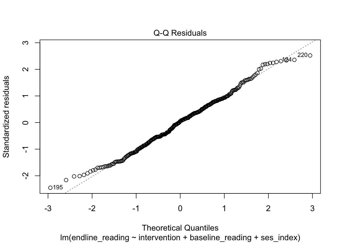
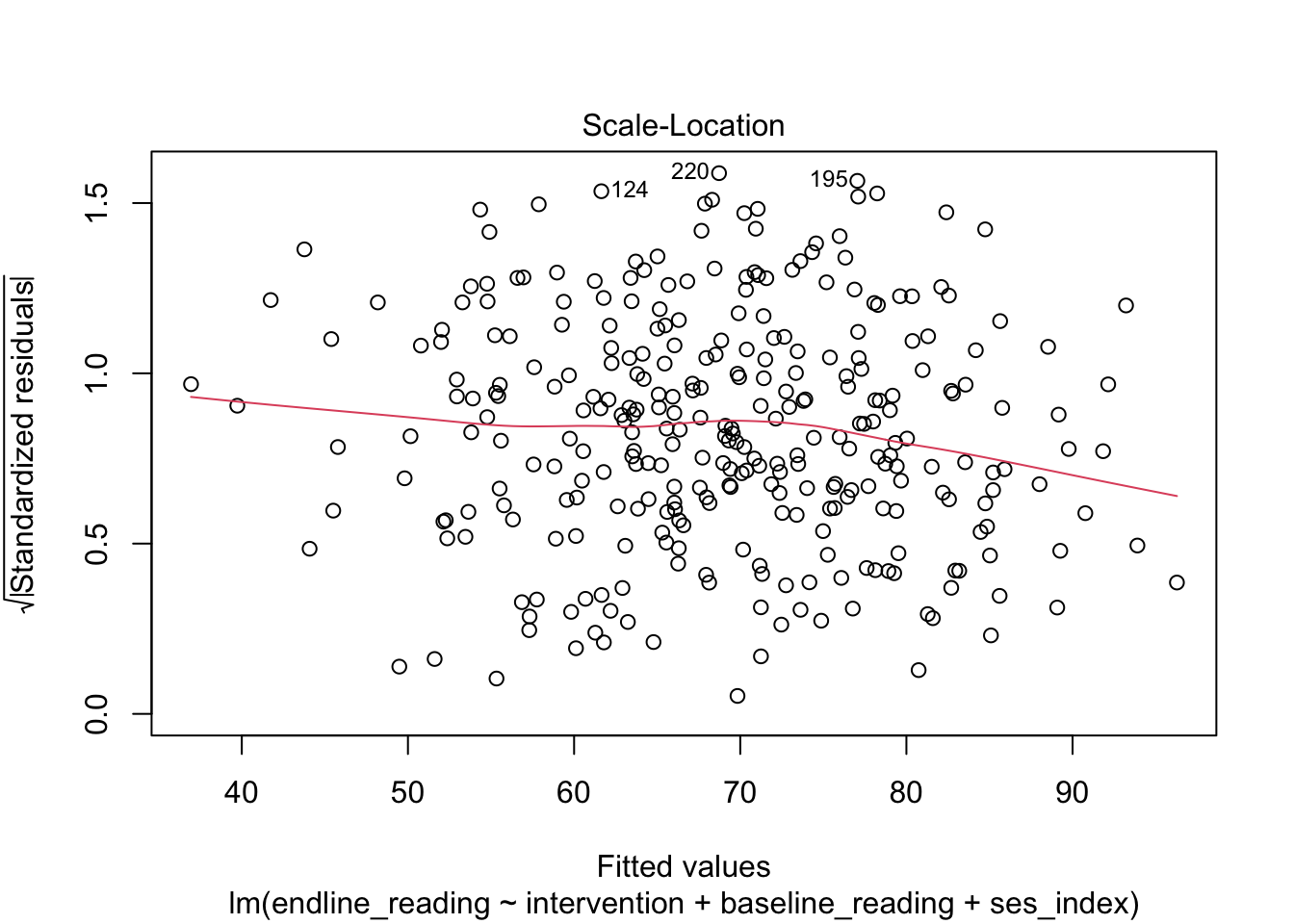
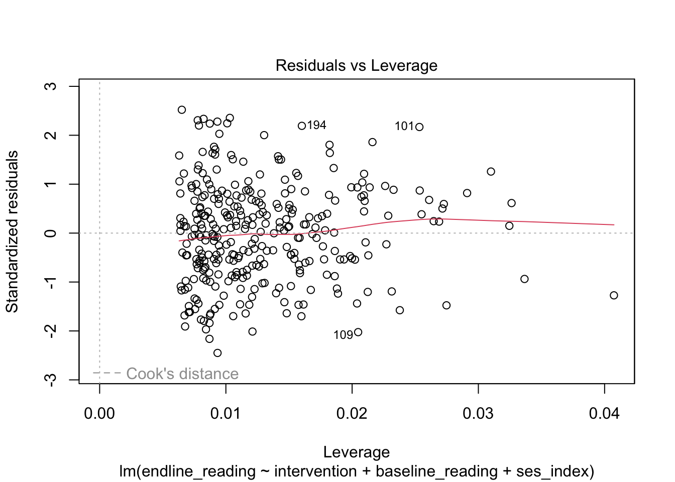
Checking the model
Use the plots to look for strong non-linearity, unequal residual spread, or unusual observations that dominate the result.
plot(score_model)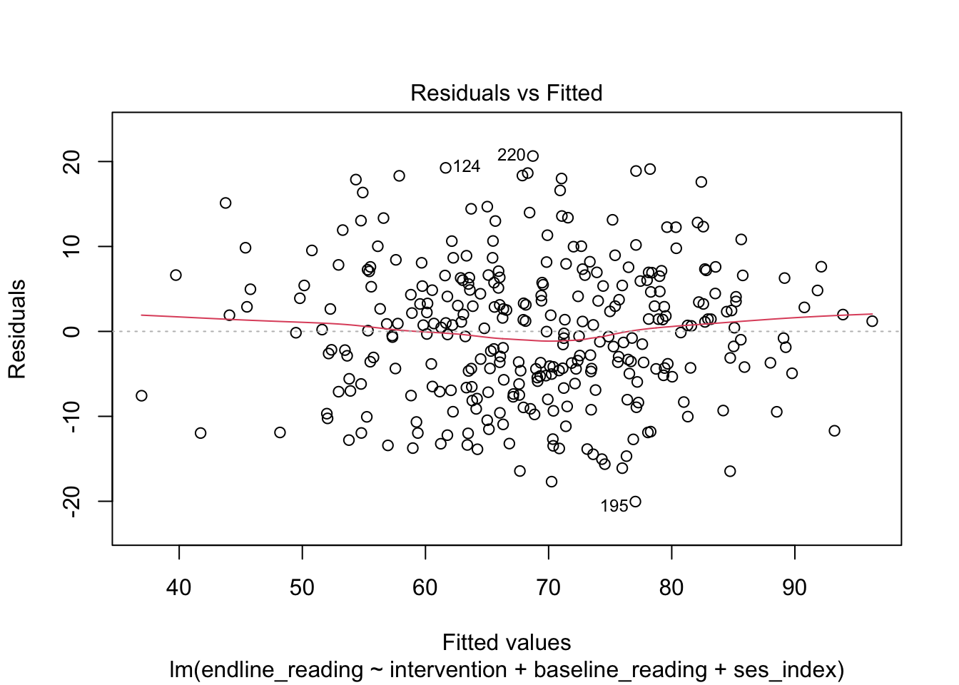
11 Adjusted Benchmark Attainment: Logistic Regression
Question
Which factors are associated with the probability of reaching the reading benchmark?
Logistic regression is used when the outcome is yes/no. Here the yes/no outcome is benchmark attainment. This section shows how the same education question can be reported as a probability-style achievement result rather than only as a mean score difference.
Hypotheses for the programme coefficient
H0: After accounting for baseline reading and attendance, the programme does not change the odds of reaching the benchmark. In odds-ratio terms, OR = 1.
H1: After accounting for baseline reading and attendance, the programme is associated with different odds of reaching the benchmark. In odds-ratio terms, OR is not 1.
This keeps the hypothesis tied to the yes/no outcome: reaching or not reaching the benchmark.
Logistic regression uses the same adjustment logic as linear regression, but the outcome is binary. The model estimates effects on the log-odds scale, which is difficult to read directly. That is why the code uses exp(coef(benchmark_model)): it converts the coefficients into odds ratios. An odds ratio of 1 means no difference in odds, values above 1 mean higher odds, and values below 1 mean lower odds. The programme test is two-sided by default: it asks whether the odds ratio differs from 1, not only whether it is greater than 1.
benchmark_model <- glm(
  met_benchmark ~ intervention + baseline_reading + attendance_rate,
  data = workflow,
  family = binomial()
)

summary(benchmark_model)
Call:
glm(formula = met_benchmark ~ intervention + baseline_reading +
    attendance_rate, family = binomial(), data = workflow)

Coefficients:
                 Estimate Std. Error z value Pr(>|z|)
(Intercept)      -9.92026    1.82047  -5.449 5.06e-08 ***
intervention      0.92275    0.32800   2.813   0.0049 **
baseline_reading  0.13919    0.01893   7.354 1.92e-13 ***
attendance_rate   0.03719    0.01929   1.928   0.0538 .
---
Signif. codes:  0 '***' 0.001 '**' 0.01 '*' 0.05 '.' 0.1 ' ' 1

(Dispersion parameter for binomial family taken to be 1)

    Null deviance: 357.34  on 311  degrees of freedom
Residual deviance: 250.42  on 308  degrees of freedom
AIC: 258.42

Number of Fisher Scoring iterations: 5exp(coef(benchmark_model)) (Intercept) intervention baseline_reading attendance_rate
4.916828e-05 2.516213e+00 1.149341e+00 1.037886e+00 exp(confint.default(benchmark_model)) 2.5 % 97.5 %
(Intercept) 1.387063e-06 0.001742906
intervention 1.322968e+00 4.785697611
baseline_reading 1.107488e+00 1.192775912
attendance_rate 9.993846e-01 1.077871528Output to look at
- The intervention odds ratio: adjusted difference in the odds of reaching the benchmark.
- The confidence interval: whether the plausible range sits mostly above, below, or across 1.
- The p-value: evidence against an odds ratio of 1.
- The baseline and attendance coefficients: whether prior achievement and attendance are also associated with benchmark attainment.
- The interpretation: odds ratios are not the same as percentage-point differences or probabilities.
Example write-up
After accounting for baseline reading and attendance, learners in the intervention group had higher odds of reaching the reading benchmark than learners in the comparison group, OR = 2.52, 95% CI [1.32, 4.79], p = .005. This means that programme participation was associated with substantially higher benchmark attainment, even after accounting for learners’ starting reading scores and attendance.
Plain-language reminder
An odds ratio of 1 means no difference in odds. Values above 1 indicate higher odds, and values below 1 indicate lower odds. If the audience needs a programme decision, also report predicted probabilities or percentages where possible.
12 Reporting Checklist
Before writing the result
- State the education question the analysis answers.
- Explain why that method fits the outcome: scale score, group mean, category, association, adjusted score, or benchmark attainment.
- Report the result on the scale readers understand: points, percentages, odds ratios, or correlations.
- Include the estimate, confidence interval, p-value, and sample size where relevant.
- For adjusted models, name the variables included in the adjustment.
- For logistic regression, do not describe odds ratios as if they were direct probability or percentage-point changes.
- Separate statistical evidence from practical importance.
- Do not make causal claims unless the design supports them.
- Explain measurement validation before using a constructed scale.
13 Using This In Your Own Paper
The point is not that every paper must contain every method on this page. The point is that the method should follow the research claim.
| If your paper needs to claim… | Use this part of the workflow | What the reader should see |
|---|---|---|
| The dataset is ready for analysis | Data validation | Coding, missing values, group sizes, and sensible ranges |
| A questionnaire scale is defensible | Measurement validation | Reliability, factor loadings, and the decision to create a scale |
| One group appears higher than another | Descriptive results and t-test | Means, standard deviations, mean difference, confidence interval |
| Outcomes differ across several settings | ANOVA | Group means, overall test, and follow-up comparisons |
| Two continuous variables move together | Correlation | Correlation coefficient, confidence interval, and cautious association language |
| A benchmark outcome differs by group | Chi-square | Percentages in each group and the test of association |
| A programme difference remains after adjustment | Linear regression | Adjusted coefficient, confidence interval, p-value, and substantive interpretation |
| A yes/no outcome needs adjusted analysis | Logistic regression | Odds ratio, confidence interval, p-value, and plain-language meaning |
Participants can use the same structure in their own research: start with the research question, choose the section that matches the outcome and claim, copy the short code, then adapt the example write-up using their own results.
Core reporting sentence
Across these examples, the strongest paper-ready result is the adjusted regression finding: learners who received the reading programme scored about 6.37 points higher on the endline reading assessment than comparable learners in the comparison group, 95% CI [4.52, 8.21], p < .001. Substantively, this suggests that the programme is associated with meaningful improvement in reading achievement, while the causal strength of that claim depends on how the intervention was assigned.
14 Link Back to Bayesian Analysis
This frequentist workflow is not a rejection of Bayesian analysis. It gives participants a clear route through the methods they already use: validation, description, analysis, checking, and reporting. The Bayesian notebooks then build from that familiar route by asking different uncertainty questions, especially questions about how plausible different effects or success rates are after the evidence is considered.
The practical bridge is this: frequentist analysis helps participants test differences, estimate associations, and report confidence intervals in familiar ways. Bayesian analysis then asks what the evidence implies about the quantities they care about, such as the probability that a programme clears a meaningful benchmark. Both routes are useful when the research question is kept visible.